County trends in insecticide use
Maggie Douglas
Last updated: 2019-11-02
Purpose
This code examines trends in absolute and toxicity-adjusted pesticide use among counties, by USDA farm resource region.
Data sources
Pesticide data is from the USGS National Pesticide Synthesis Project. Toxicity data were generated as describe in the code here, here and here. Data on county acreage are from the US Agricultural Census, as described here. Farm resource regions are from USDA-ERS, as described here.
Libraries and functions
library(tidyverse)
library(gridExtra)
library(GGally)
library(trend)
Load data
pest <- read.csv("../output_big/bee_tox_index_cty.csv", colClasses=c("fips"="character"))
pest_class <- read.csv("../output_big/bee_tox_index_cty_class.csv", colClasses=c("fips"="character"))
Calculate key indicators
pest_ind_cty <- pest %>%
  filter(YEAR %in% c(1997,2002,2007,2012)) %>%
  mutate(crop_perc = (crop_ha/ha)*100,
         trt_perc = (trt_ins_ha/crop_ha)*100,
         extent_ha = trt_ins_ha,
         extent_perc = (trt_ins_ha/ha)*100,
         app_rate = kg_low/(extent_ha),
         ct_potency = ct_tox_bil_low/kg_low,
         or_potency = or_tox_bil_low/kg_low,
         ct_intensity = ct_tox_bil_low/extent_ha,
         or_intensity = or_tox_bil_low/extent_ha,
         ct_ha = ct_tox_bil_low/(ha),
         or_ha = or_tox_bil_low/(ha))

pest_ind_cty_long <- pest_ind_cty %>%
  gather(key = "var", value = "value", kg_low:or_ha)
Warning: attributes are not identical across measure variables;
they will be droppedpest_ind_cty_97 <- pest_ind_cty_long %>%
filter(YEAR==1997) %>%
rename(value_97 = value) %>%
select(fips, var, value_97)
pest_cty_chg <- pest_ind_cty_long %>%
left_join(pest_ind_cty_97, by = c("fips","var")) %>%
mutate(value = as.numeric(value),
value_97 = as.numeric(value_97),
perc_chg = ((value-value_97)/value_97)*100,
RR = value/value_97,
logRR = log10(RR))Warning: NAs introduced by coercionWarning: NAs introduced by coercionpest_ind_reg <- pest %>%
group_by(YEAR, region_name) %>%
summarise(crop_ha = sum(crop_ha, na.rm = TRUE),
trt_ins_ha = sum(trt_ins_ha, na.rm = TRUE),
kg_low = sum(kg_low, na.rm = TRUE),
or_tox_bil_low = sum(or_tox_bil_low, na.rm = TRUE),
ct_tox_bil_low = sum(ct_tox_bil_low, na.rm = TRUE),
ha = sum(ha, na.rm = TRUE),
crop_perc = (crop_ha/ha)*100,
trt_perc = (trt_ins_ha/crop_ha)*100,
extent_ha = trt_ins_ha,
extent_perc = (trt_ins_ha/ha)*100,
app_rate = kg_low/(extent_ha),
ct_potency = ct_tox_bil_low/kg_low,
or_potency = or_tox_bil_low/kg_low,
ct_intensity = ct_tox_bil_low/extent_ha,
or_intensity = or_tox_bil_low/extent_ha,
ct_ha = ct_tox_bil_low/ha,
or_ha = or_tox_bil_low/ha) %>%
na.omit() %>%
gather(key = "var", value = "value", crop_ha:or_ha)
pest_ind_97 <- pest_ind_reg %>%
filter(YEAR==1997) %>%
rename(value_97 = value) %>%
ungroup() %>%
select(-YEAR)
pest_reg_chg <- pest_ind_reg %>%
left_join(pest_ind_97, by = c("var", "region_name")) %>%
mutate(perc_chg = ((value-value_97)/value_97)*100,
RR = value/value_97,
logRR = log10(RR))
pest_ind_nat <- pest %>%
group_by(YEAR) %>%
summarise(crop_ha = sum(crop_ha, na.rm = TRUE),
trt_ins_ha = sum(trt_ins_ha, na.rm = TRUE),
kg_low = sum(kg_low, na.rm = TRUE),
or_tox_bil_low = sum(or_tox_bil_low, na.rm = TRUE),
ct_tox_bil_low = sum(ct_tox_bil_low, na.rm = TRUE),
ha = sum(ha, na.rm = TRUE),
crop_perc = (crop_ha/ha)*100,
trt_perc = (trt_ins_ha/crop_ha)*100,
extent_ha = trt_ins_ha,
extent_perc = (trt_ins_ha/ha)*100,
app_rate = kg_low/(extent_ha),
ct_potency = ct_tox_bil_low/kg_low,
or_potency = or_tox_bil_low/kg_low,
ct_intensity = ct_tox_bil_low/extent_ha,
or_intensity = or_tox_bil_low/extent_ha,
ct_ha = ct_tox_bil_low/ha,
or_ha = or_tox_bil_low/ha) %>%
na.omit() %>%
gather(key = "var", value = "value", crop_ha:or_ha)
pest_nat_97 <- pest_ind_nat %>%
filter(YEAR==1997) %>%
rename(value_97 = value) %>%
ungroup() %>%
select(-YEAR)
pest_nat_chg <- pest_ind_nat %>%
left_join(pest_nat_97, by = c("var")) %>%
mutate(perc_chg = ((value-value_97)/value_97)*100,
RR = value/value_97,
logRR = log10(RR))Descriptives
# top 10% of counties - contact basis
top10_ct <- pest_ind_cty %>%
  filter(YEAR == 2012) %>%
  mutate(percentile = ntile(ct_tox_bil_low, 10)) %>%
  group_by(percentile) %>%
  summarise(ct_tox_bil_low = sum(ct_tox_bil_low, na.rm=T))

(top10_ct$ct_tox_bil_low[top10_ct$percentile == 10])/sum(top10_ct$ct_tox_bil_low)
[1] 0.5451843# top 10% of counties - oral basis
top10_or <- pest_ind_cty %>%
filter(YEAR == 2012) %>%
mutate(percentile = ntile(or_tox_bil_low, 10)) %>%
group_by(percentile) %>%
summarise(or_tox_bil_low = sum(or_tox_bil_low, na.rm=T))
(top10_or$or_tox_bil_low[top10_or$percentile == 10])/sum(top10_or$or_tox_bil_low)[1] 0.4836745# change in contact toxic load
cty_chg <- pest_cty_chg %>%
filter(YEAR == 2012 & var %in% c("ct_tox_bil_low", "or_tox_bil_low")) %>%
group_by(var) %>%
summarise(median_RR = median(RR, na.rm=T),
low_quant_RR = quantile(RR, 1/4, na.rm=T),
high_quant_RR = quantile(RR, 3/4, na.rm = T),
median_perc = median(perc_chg, na.rm=T),
low_quant_perc = quantile(perc_chg, 1/4, na.rm=T),
high_quant_perc = quantile(perc_chg, 3/4, na.rm = T),
count_inc = (length(perc_chg[perc_chg > 0]))/length(perc_chg),
count_dec = (length(perc_chg[perc_chg < 0]))/length(perc_chg))
# contribution of neonics to total
pest_class_sum <- pest_class %>%
group_by(YEAR, class_short) %>%
summarise(kg_low = sum(kg_low, na.rm = T),
ct_tox_bil_low = sum(ct_tox_bil_low, na.rm = T),
or_tox_bil_low = sum(or_tox_bil_low, na.rm = T))Warning: Factor `class_short` contains implicit NA, consider using
`forcats::fct_explicit_na`pest_sum <- pest_class %>%
group_by(YEAR) %>%
summarise(kg_low = sum(kg_low, na.rm = T),
ct_tox_bil_low = sum(ct_tox_bil_low, na.rm = T),
or_tox_bil_low = sum(or_tox_bil_low, na.rm = T))
ct_neo <- na.omit(pest_class_sum$ct_tox_bil_low[pest_class_sum$YEAR==2012 &
pest_class_sum$class_short=="NEO"])
or_neo <- na.omit(pest_class_sum$or_tox_bil_low[pest_class_sum$YEAR==2012 &
pest_class_sum$class_short=="NEO"])
ct_tot <- pest_sum$ct_tox_bil_low[pest_sum$YEAR==2012]
or_tot <- pest_sum$or_tox_bil_low[pest_sum$YEAR==2012]
ct_neo/ct_tot[1] 0.2993454 NAor_neo/or_tot[1] 0.9809824 NAGraph insecticide trends by class (Figure 2)
pest_class_long <- pest_class %>%
  filter(cat == "I") %>%
  select(YEAR, fips, class_short, kg_low, ct_tox_bil_low, or_tox_bil_low) %>%
  gather(key = "var",
         value = "amount",
         kg_low:or_tox_bil_low)

pest_class_long$var <- fct_relevel(pest_class_long$var, "kg_low", "ct_tox_bil_low", "or_tox_bil_low")

var_names <- list(
  'kg_low'="Weight (mil kg)",
  'ct_tox_bil_low'=expression('Contact toxic load (10'^15*' bee LD'[50]*'s)'),
  'or_tox_bil_low'=expression('Oral toxic load (10'^15*' bee LD'[50]*'s)')
)

var_labeller <- function(variable,value){
  return(var_names[value])
}

text_lab <- data.frame(
  label = c("a", "b", "c"),
  var   = c("kg_low", "ct_tox_bil_low", "or_tox_bil_low")
)

ggplot(filter(pest_class_long, YEAR > 1996 & YEAR < 2013),
       aes(fill = class_short, x = YEAR, y = amount/10^6)) +
  geom_col() +
  facet_wrap(~var, scales = "free_y",
         strip.position = "left",
         labeller = var_labeller) +
  ylab(NULL) +
  xlab(NULL) +
  theme_classic(base_size=18) +
  theme(strip.background = element_blank(),
        strip.placement = "outside") +
  scale_fill_brewer(palette = "Set3") +
  guides(fill=guide_legend(title=NULL))
Warning: The labeller API has been updated. Labellers taking `variable`and
`value` arguments are now deprecated. See labellers documentation.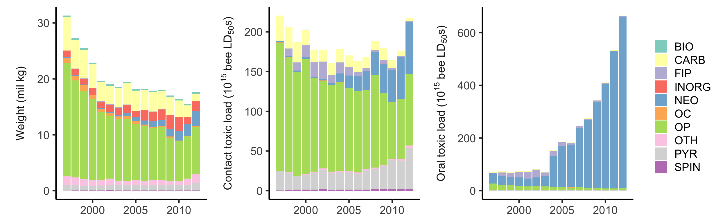
Test for national trends
pest_sum_focal <- filter(pest_sum, YEAR > 1996 & YEAR < 2013)
mk.test(pest_sum_focal$kg_low)
    Mann-Kendall trend test

data:  pest_sum_focal$kg_low
z = -4.7274, n = 16, p-value = 2.275e-06
alternative hypothesis: true S is not equal to 0
sample estimates:
           S         varS          tau
-106.0000000  493.3333333   -0.8833333
mk.test(pest_sum_focal$ct_tox_bil_low)
    Mann-Kendall trend test

data:  pest_sum_focal$ct_tox_bil_low
z = -1.3957, n = 16, p-value = 0.1628
alternative hypothesis: true S is not equal to 0
sample estimates:
          S        varS         tau
-32.0000000 493.3333333  -0.2666667
mk.test(pest_sum_focal$or_tox_bil_low)
    Mann-Kendall trend test

data:  pest_sum_focal$or_tox_bil_low
z = 4.5473, n = 16, p-value = 5.435e-06
alternative hypothesis: true S is not equal to 0
sample estimates:
       S     varS      tau
102.0000 493.3333   0.8500
Test for regional trends
pest_sum_reg <- pest_class %>%
  filter(YEAR > 1996 & YEAR < 2013) %>%
  group_by(YEAR, region_name) %>%
  summarise(kg_low = sum(kg_low, na.rm = T),
            ct_tox_bil_low = sum(ct_tox_bil_low, na.rm = T),
            or_tox_bil_low = sum(or_tox_bil_low, na.rm = T)) %>%
  arrange(region_name) %>%
  ungroup()

reg_list <- split(pest_sum_reg, pest_sum_reg$region_name)

mk_ct <- function(x){
  mk.test(x$ct_tox_bil_low)
}

mk_or <- function(x){
  mk.test(x$or_tox_bil_low)
}

results_ct <- lapply(reg_list, FUN = mk_ct)
results_or <- lapply(reg_list, FUN = mk_or)
Summarize X region, 1997-2012 (Figure S3)
reg_12 <- pest_reg_chg %>%
  filter(YEAR==2012 &
           var %in% c("or_potency","ct_potency", "or_intensity", "ct_intensity",
                      "crop_ha","trt_perc","app_rate","extent_ha",
                      "ct_tox_bil_low", "or_tox_bil_low")) %>%
  mutate(grp = ifelse(var %in% c("crop_ha", "trt_perc"), "Contributors to extent",
                      ifelse(var %in% c("extent_ha"), "Extent",
                      ifelse(var %in% c("app_rate", "ct_potency", "or_potency"), "Contributors to intensity",
                             ifelse(var %in% c("ct_intensity", "or_intensity"), "Intensity",
                             "Toxic load"))))) %>%
  mutate(fill_grp = ifelse(var %in% c("crop_ha", "trt_perc", "extent_ha", "app_rate"), "one",
                           ifelse(var %in% c("ct_potency", "ct_intensity", "ct_tox_bil_low"), "two",
                                  "three"))) %>%
  ungroup()

x_labels <- c("crop_ha" = "Total cropland (ha)",
              "trt_perc" = "Cropland treated (%)",
              "extent_ha" = "Area treated (ha)",
              "app_rate" = "Application rate (kg/ha)",
              "ct_potency" = "Contact potency (bee LD50s/kg)",
              "or_potency" = "Oral potency (bee LD50s/kg)",
              "ct_intensity" = "Contact (bee LD50s/trt-ha)",
              "or_intensity" = "Oral (bee LD50s/trt-ha)",
              "ct_tox_bil_low" = "Contact (bee LD50s)",
              "or_tox_bil_low" = "Oral (bee LD50s)")

reg_12$grp <- factor(reg_12$grp, levels = c("Contributors to extent",
                                            "Extent",
                                            "Contributors to intensity",
                                            "Intensity",
                                            "Toxic load"))

# desired breaks
brk <- c(100,30,10,3,1,.3,.1)
lgbrk <- log10(brk)

# colors for bars
col <- c("gray","darkorange","red")

ggplot(data = reg_12, aes(x = var, y = logRR, fill = fill_grp)) +
  geom_bar(stat = "identity", colour = "black", width = 0.75) +
  facet_grid(region_name~grp, scales = "free_x", space = "free",
             labeller = label_wrap_gen(width=10)) +
  geom_abline(yintercept = 0, slope = 0, lty = 2) +
  theme_classic() +
  scale_x_discrete(labels = x_labels) +
  scale_y_continuous(breaks = lgbrk, labels = brk) +
  scale_fill_manual(values = col) +
  theme(axis.line=element_blank(),
        axis.text.x = element_text(angle = 60, hjust = 1),
        legend.position = "none",
        strip.background = element_blank(),
        panel.border = element_rect(colour="black", size = 0.5, fill=NA)) +
  xlab("") +
  ylab("Fold-change, 1997-2012")
Warning: Ignoring unknown parameters: yintercept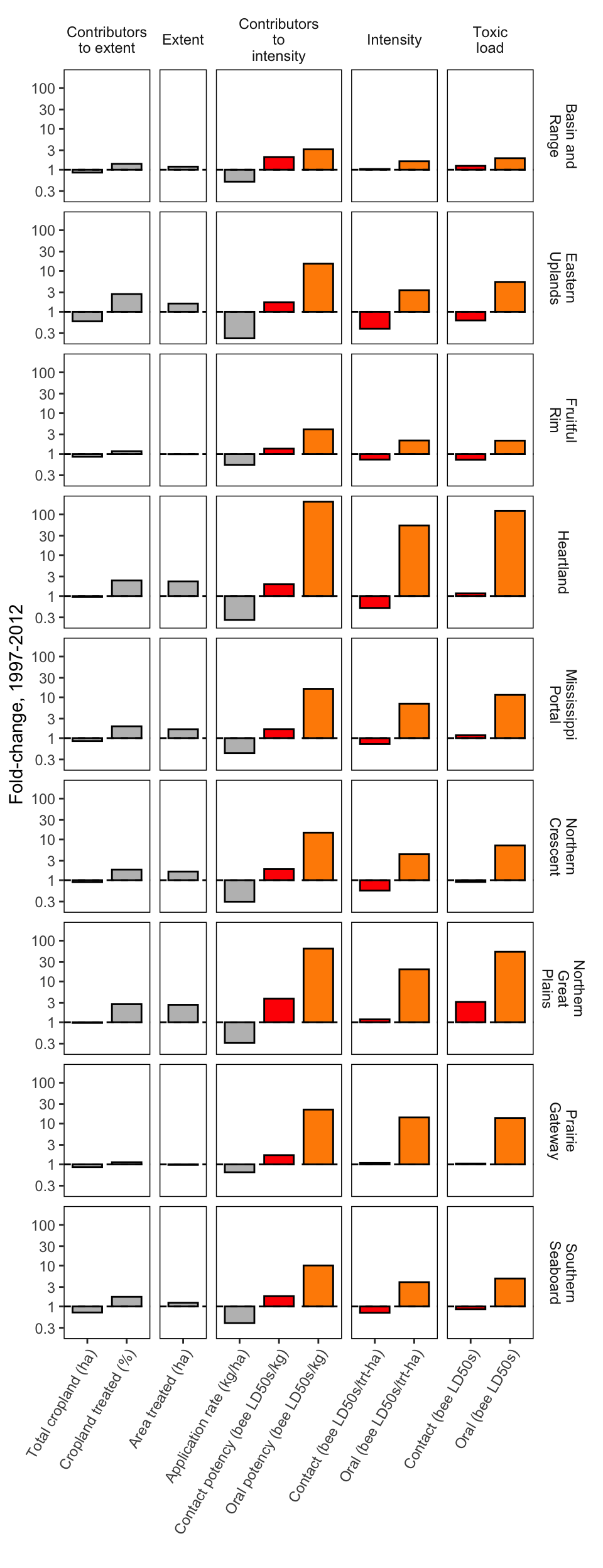
Summarize nationally, 1997-2012
nat_12 <- pest_nat_chg %>%
  filter(YEAR==2012 &
           var %in% c("or_potency","ct_potency", "or_intensity", "ct_intensity",
                      "crop_ha","trt_perc","app_rate","extent_ha",
                      "ct_tox_bil_low", "or_tox_bil_low")) %>%
  mutate(grp = ifelse(var %in% c("crop_ha", "trt_perc"), "Contributors to extent",
                      ifelse(var %in% c("extent_ha"), "Extent",
                      ifelse(var %in% c("app_rate", "ct_potency", "or_potency"), "Contributors to intensity",
                             ifelse(var %in% c("ct_intensity", "or_intensity"), "Intensity",
                             "Toxic load"))))) %>%
  mutate(fill_grp = ifelse(var %in% c("crop_ha", "trt_perc", "extent_ha", "app_rate"), "one",
                           ifelse(var %in% c("ct_potency", "ct_intensity", "ct_tox_bil_low"), "two",
                                  "three")),
         region_name = "National (contiguous U.S.)") %>%
  ungroup()

x_labels <- c("crop_ha" = "Total cropland (ha)",
              "trt_perc" = "Cropland treated (%)",
              "extent_ha" = "Area treated (ha)",
              "app_rate" = "Application rate (kg/ha)",
              "ct_potency" = "Contact potency (bee LD50s/kg)",
              "or_potency" = "Oral potency (bee LD50s/kg)",
              "ct_intensity" = "Contact (bee LD50s/trt-ha)",
              "or_intensity" = "Oral (bee LD50s/trt-ha)",
              "ct_tox_bil_low" = "Contact (bee LD50s)",
              "or_tox_bil_low" = "Oral (bee LD50s)")

nat_12$grp <- factor(nat_12$grp, levels = c("Contributors to extent",
                                            "Extent",
                                            "Contributors to intensity",
                                            "Intensity",
                                            "Toxic load"))

# desired breaks
brk <- c(100,30,10,3,1,.3,.1)
lgbrk <- log10(brk)

# colors for bars
col <- c("gray","darkorange","red")

ggplot(data = nat_12, aes(x = var, y = logRR, fill = fill_grp)) +
  geom_bar(stat = "identity", colour = "black", width = 0.75) +
  facet_grid(.~grp, scales = "free_x", space = "free") +
  geom_abline(yintercept = 0, slope = 0, lty = 2) +
  theme_classic() +
  scale_x_discrete(labels = x_labels) +
  scale_y_continuous(breaks = lgbrk, labels = brk) +
  scale_fill_manual(values = col) +
  theme(axis.line=element_blank(),
        axis.text.x = element_text(angle = 60, hjust = 1),
        legend.position = "none",
        strip.background = element_blank(),
        panel.border = element_rect(colour="black", size = 0.5, fill=NA)) +
  xlab("") +
  ylab("Fold-change, 1997-2012")
Warning: Ignoring unknown parameters: yintercept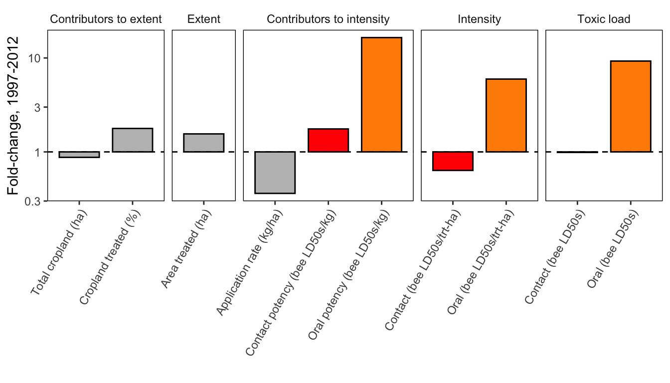
Summary figure, 1997-2012 (Figure 4)
sum_12 <- rbind(reg_12, nat_12) %>%
  filter(region_name %in% c("National (contiguous U.S.)",
                            "Heartland",
                            "Northern Great Plains"))

sum_12$region_name <- factor(sum_12$region_name,
                             levels = c("National (contiguous U.S.)",
                                        "Heartland",
                                        "Northern Great Plains"))

x_labels <- c("crop_ha" = "Total cropland (ha)",
              "trt_perc" = "Cropland treated (%)",
              "extent_ha" = "Area treated (ha)",
              "app_rate" = "Application rate (kg/ha)",
              "ct_potency" = "Contact potency (bee LD50s/kg)",
              "or_potency" = "Oral potency (bee LD50s/kg)",
              "ct_intensity" = "Contact (bee LD50s/trt-ha)",
              "or_intensity" = "Oral (bee LD50s/trt-ha)",
              "ct_tox_bil_low" = "Contact (bee LD50s)",
              "or_tox_bil_low" = "Oral (bee LD50s)")

sum_12$grp <- factor(sum_12$grp, levels = c("Contributors to extent",
                                            "Extent",
                                            "Contributors to intensity",
                                            "Intensity",
                                            "Toxic load"))

# desired breaks
brk <- c(100,30,10,3,1,.3,.1)
lgbrk <- log10(brk)

# colors for bars
col <- c("gray","darkorange","red")

ggplot(data = sum_12, aes(x = var, y = logRR, fill = fill_grp)) +
  geom_bar(stat = "identity", colour = "black", width = 0.75) +
  facet_grid(region_name~grp, scales = "free_x", space = "free",
             labeller = label_wrap_gen(width=18)) +
  geom_abline(yintercept = 0, slope = 0, lty = 2) +
  theme_classic() +
  scale_x_discrete(labels = x_labels) +
  scale_y_continuous(breaks = lgbrk, labels = brk) +
  scale_fill_manual(values = col) +
  theme(axis.line=element_blank(),
        axis.text.x = element_text(angle = 60, hjust = 1),
        legend.position = "none",
        strip.background = element_blank(),
        panel.border = element_rect(colour="black", size = 0.5, fill=NA)) +
  xlab("") +
  ylab("Fold-change, 1997-2012")
Warning: Ignoring unknown parameters: yintercept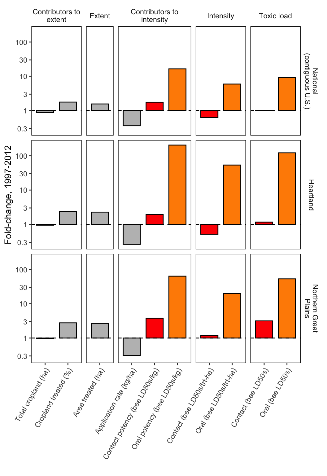
Summarize 2012 values in a table (Table 1)
reg_12_tab <- pest_ind_reg %>%
  filter(YEAR == 2012) %>%
  spread(key = var, value = value) %>%
  mutate(ha_mil = ha/10^6) %>%
  select(YEAR, region_name, ha_mil, extent_perc, ct_intensity, or_intensity,
         ct_ha, or_ha) %>%
  mutate(ha_mil = round(ha_mil, digits = 0),
         extent_perc = round(extent_perc, digits = 1),
         ct_intensity = round(ct_intensity, digits = 0),
         or_intensity = round(or_intensity, digits = 0),
         ct_ha = round(ct_ha, digits = 2),
         or_ha = round(or_ha, digits = 2))

nat_12_tab <- pest_ind_nat %>%
  filter(YEAR == 2012) %>%
  spread(key = var, value = value) %>%
  mutate(ha_mil = ha/10^6,
         region_name = "Contiguous U.S.") %>%
  select(YEAR, region_name, ha_mil, extent_perc, ct_intensity, or_intensity,
         ct_ha, or_ha) %>%
  mutate(ha_mil = round(ha_mil, digits = 0),
         extent_perc = round(extent_perc, digits = 1),
         ct_intensity = round(ct_intensity, digits = 0),
         or_intensity = round(or_intensity, digits = 0),
         ct_ha = round(ct_ha, digits = 2),
         or_ha = round(or_ha, digits = 2))

table <- bind_rows(reg_12_tab, nat_12_tab)
Warning in bind_rows_(x, .id): binding factor and character vector,
coercing into character vectorWarning in bind_rows_(x, .id): binding character and factor vector,
coercing into character vectorExport data
write.csv(pest_ind_cty, "../output_big/bee_tox_cty_indicators.csv", row.names=FALSE)Session information
sessionInfo()R version 3.6.1 (2019-07-05)
Platform: x86_64-apple-darwin15.6.0 (64-bit)
Running under: macOS High Sierra 10.13.6
Matrix products: default
BLAS: /Library/Frameworks/R.framework/Versions/3.6/Resources/lib/libRblas.0.dylib
LAPACK: /Library/Frameworks/R.framework/Versions/3.6/Resources/lib/libRlapack.dylib
locale:
[1] en_US.UTF-8/en_US.UTF-8/en_US.UTF-8/C/en_US.UTF-8/en_US.UTF-8
attached base packages:
[1] stats graphics grDevices utils datasets methods base
other attached packages:
[1] trend_1.1.1 GGally_1.4.0 gridExtra_2.3 forcats_0.4.0
[5] stringr_1.4.0 dplyr_0.8.3 purrr_0.3.2 readr_1.3.1
[9] tidyr_0.8.3 tibble_2.1.3 ggplot2_3.2.0 tidyverse_1.2.1
loaded via a namespace (and not attached):
[1] tidyselect_0.2.5 xfun_0.8 reshape2_1.4.3
[4] haven_2.1.1 lattice_0.20-38 colorspace_1.4-1
[7] generics_0.0.2 vctrs_0.2.0 htmltools_0.3.6
[10] yaml_2.2.0 rlang_0.4.0 pillar_1.4.2
[13] glue_1.3.1 withr_2.1.2 RColorBrewer_1.1-2
[16] modelr_0.1.4 readxl_1.3.1 plyr_1.8.4
[19] munsell_0.5.0 gtable_0.3.0 cellranger_1.1.0
[22] rvest_0.3.4 evaluate_0.14 labeling_0.3
[25] knitr_1.23 broom_0.5.2 Rcpp_1.0.1
[28] scales_1.0.0 backports_1.1.4 jsonlite_1.6
[31] hms_0.5.0 digest_0.6.20 stringi_1.4.3
[34] grid_3.6.1 cli_1.1.0 tools_3.6.1
[37] magrittr_1.5 lazyeval_0.2.2 crayon_1.3.4
[40] pkgconfig_2.0.2 zeallot_0.1.0 xml2_1.2.0
[43] lubridate_1.7.4 extraDistr_1.8.11 assertthat_0.2.1
[46] rmarkdown_1.14 reshape_0.8.8 httr_1.4.0
[49] rstudioapi_0.10 R6_2.4.0 nlme_3.1-140
[52] compiler_3.6.1 This R Markdown site was created with workflowr