County patterns in pesticide use
Maggie Douglas
Last updated: 2019-10-25
Purpose
This code creates county maps showing insecticide use and insect toxic load, as well as change from 1997-2012.
Libraries and functions
library(tidyverse)
library(sp)
library(sf)
library(tigris)
library(RColorBrewer)
library(classInt)
Load data
pest_cty <- read.csv("../output_big/bee_tox_index_cty.csv",
                     colClasses=c("fips"="character"))
Data preparation
# reorganize data, calc key metrics, and calc change since 1997
pest_cty_org <- pest_cty %>%
  mutate(perc_crop = (crop_ha/ha)*100,
         perc_trt = (trt_ins_ha/ha)*100,
         kg_ha = kg_low/ha,
         ct_kg = ct_tox_bil_low/kg_low,
         or_kg = or_tox_bil_low/kg_low,
         ct_tox_ha = ct_tox_bil_low/ha,
         or_tox_ha = or_tox_bil_low/ha) %>%
  select(YEAR, region_name, region_code, fips, perc_crop, perc_trt, kg_ha,
         ct_kg, or_kg, ct_tox_ha, or_tox_ha) %>%
  gather(key = "var", value = "value", perc_crop:or_tox_ha)

pest_cty_97 <- pest_cty_org %>%
  filter(YEAR==1997) %>%
  rename(value_97 = value) %>%
  select(fips, var, value_97)

pest_cty_chg <- pest_cty_org %>%
  left_join(pest_cty_97, by = c("fips", "var")) %>%
  mutate(value = as.numeric(value),
         value_97 = as.numeric(value_97),
         chg = value-value_97,
         perc_chg = ((value-value_97)/value_97)*100)

pest_cty_12 <- filter(pest_cty_chg, YEAR==2012)
Load and join map data
# load county boundaries
cnty <- tigris::counties(cb = TRUE, resolution = "20m")

# convert county boundaries to sf object
# remove Hawaii, Alaska, and Puerto Rico
cnty_sf <- st_as_sf(cnty) %>%
  filter(STATEFP!="15" & STATEFP!="02" & STATEFP!="72")

# and merge with pest data
cnty_sf_join <- cnty_sf %>%
  dplyr::full_join(pest_cty_12, by = c("GEOID" = "fips")) %>%
  st_transform(crs = 5070)
Create shapefile of regions
regions <- cnty_sf_join %>%
  group_by(region_name) %>%
  summarise()
Warning: Factor `region_name` contains implicit NA, consider using
`forcats::fct_explicit_na`# store transparent color palette
clear_pal <- adjustcolor(palette(), alpha = 0)Distributions of key responses
# examine distribution of key response variables
ggplot(data = filter(pest_cty_chg, var=="perc_trt" & YEAR==2012),
                     aes(value*100)) +
  geom_histogram(bins=100) +
  theme_classic() +
  xlab("% area treated")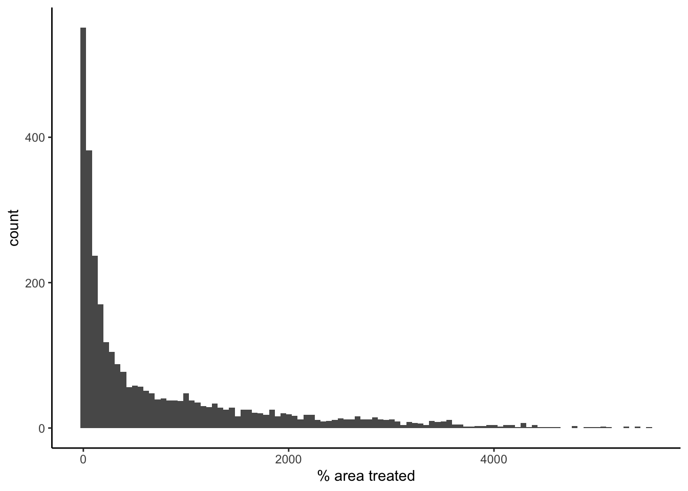
ggplot(data = filter(pest_cty_chg, var=="or_tox_ha" & YEAR==2012),
                     aes(value)) +
  geom_histogram(bins=100) +
  theme_classic() +
  xlab("Oral toxicity per ha")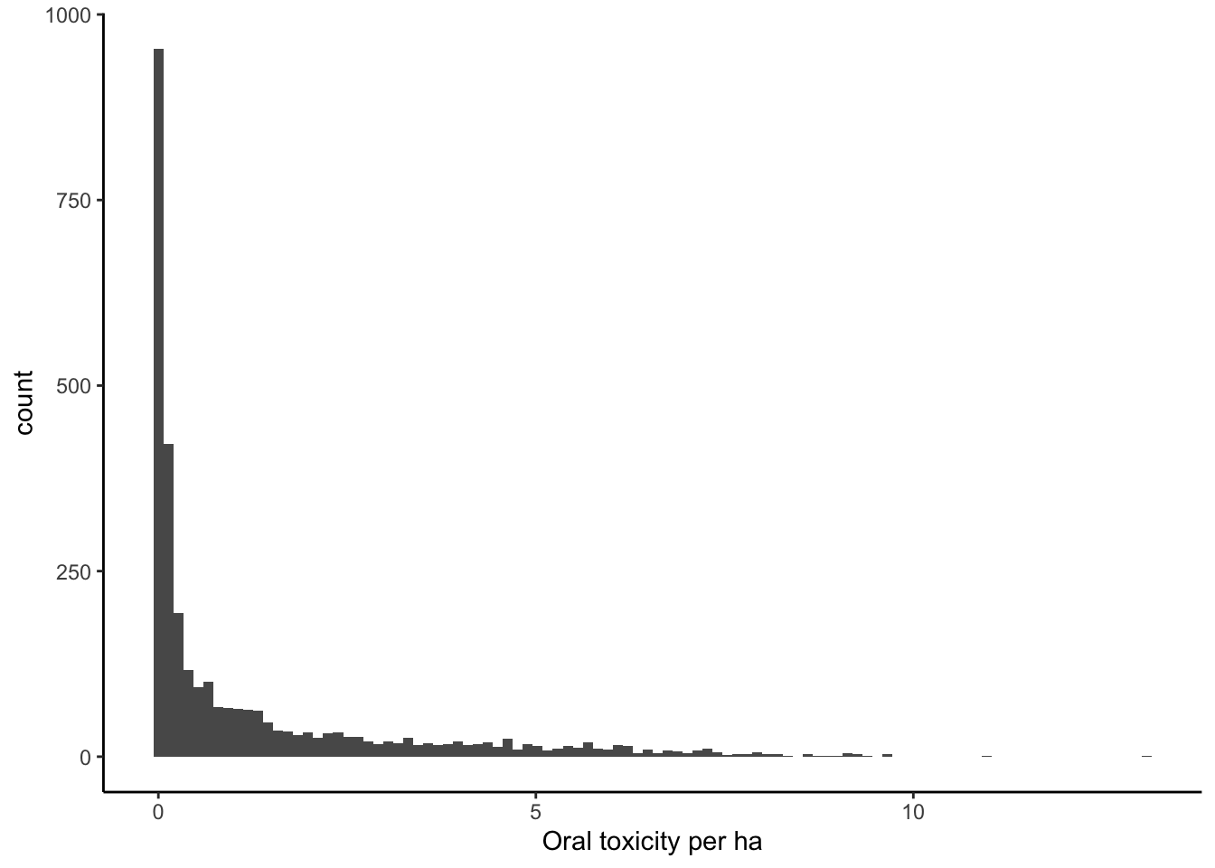
ggplot(data = filter(pest_cty_chg, var=="ct_tox_ha" & YEAR==2012),
                     aes(value)) +
  geom_histogram(bins=100) +
  theme_classic() +
  xlab("Contact toxicity per ha")
ggplot(data = filter(pest_cty_chg, var=="perc_trt" & YEAR==2012),
                     aes(chg*100)) +
  geom_histogram(bins=100) +
  theme_classic() +
  xlab("Change in area treated")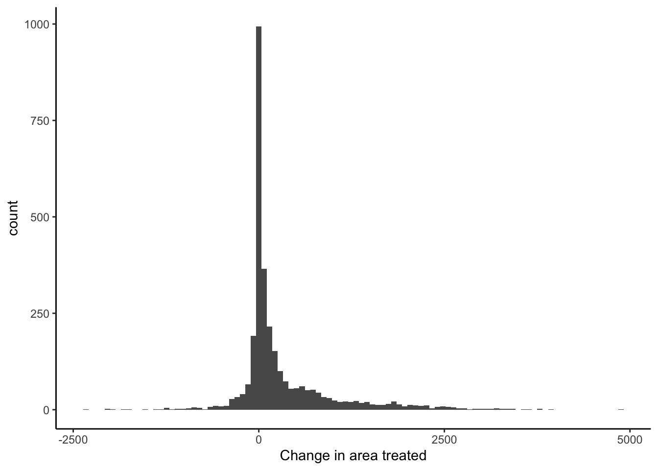
ggplot(data = filter(pest_cty_chg, var=="or_tox_ha" & YEAR==2012),
                     aes(chg)) +
  geom_histogram(bins=100) +
  theme_classic() +
  xlab("Change in oral toxicity per ha")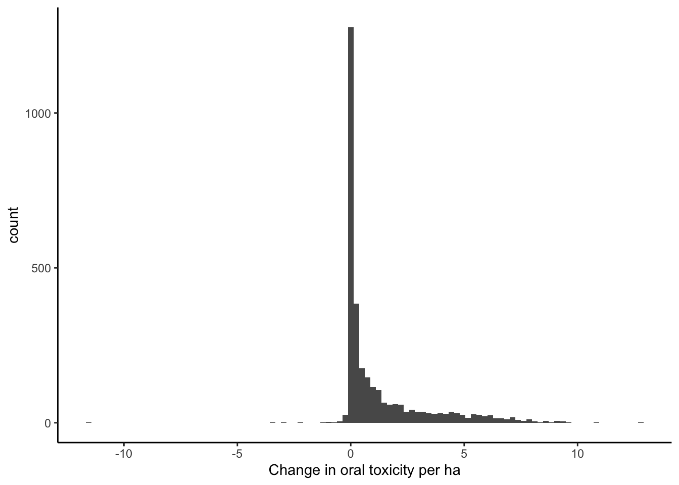
ggplot(data = filter(pest_cty_chg, var=="ct_tox_ha" & YEAR==2012),
                     aes(chg)) +
  geom_histogram(bins=100) +
  theme_classic() +
  xlab("Change in contact toxicity per ha")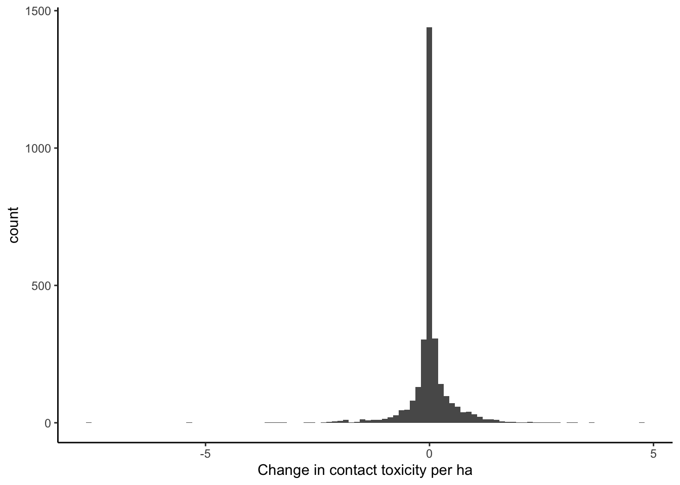
Contact toxic load 2012
my_pal <- brewer.pal(n = 6, name = "OrRd")
ct_tox_ha_12 <- filter(cnty_sf_join, var=="ct_tox_ha" & is.finite(value))

plot(ct_tox_ha_12["value"],
     pal = my_pal,
     breaks = "jenks",
     nbreaks = 6,
     main = "",
     lwd = 0.1,
     key.width = .1,
     reset=FALSE)
Warning in classInt::classIntervals(na.omit(values), min(nbreaks, n.unq), :
N is large, and some styles will run very slowly; sampling imposedUse "fisher" instead of "jenks" for larger data setsplot(regions,
main = "",
pal = clear_pal,
lwd = 0.8,
key.pos = NULL,
add=T)
title(expression(paste(bold("a"), " Contact toxic load 2012 (bil bee LD50/ha)")), adj = 0)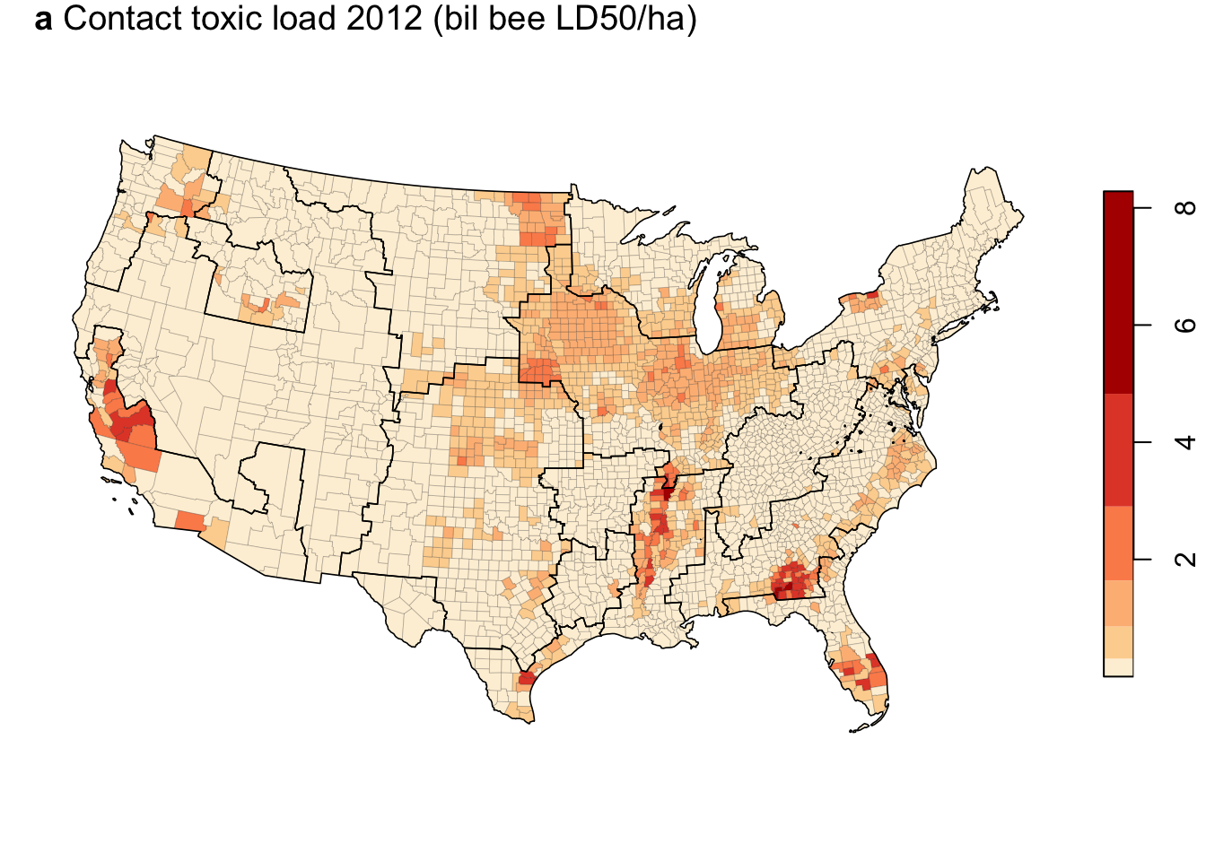
Change in contact toxic load 1997-2012
my_pal <- c("#2166AC","#67A9CF","#D1E5F0","#F7F7F7", "#FDDBC7","#EF8A62")
ct_tox_ha_12 <- filter(cnty_sf_join, var=="ct_tox_ha" & is.finite(chg))

plot(ct_tox_ha_12["chg"],
     pal = my_pal,
     breaks = "jenks",
     nbreaks = 6,
     lwd = 0.1,
     key.width = 0.1,
     main = "",
     reset=FALSE)
Warning in classInt::classIntervals(na.omit(values), min(nbreaks, n.unq), :
N is large, and some styles will run very slowly; sampling imposedUse "fisher" instead of "jenks" for larger data setsplot(regions,
main = "",
pal = clear_pal,
lwd = 0.8,
key.pos = NULL,
add=T)
title(expression(paste(bold("b"), " Change in contact toxic load, 1997-2012 (bil bee LD50/ha)")), adj = 0)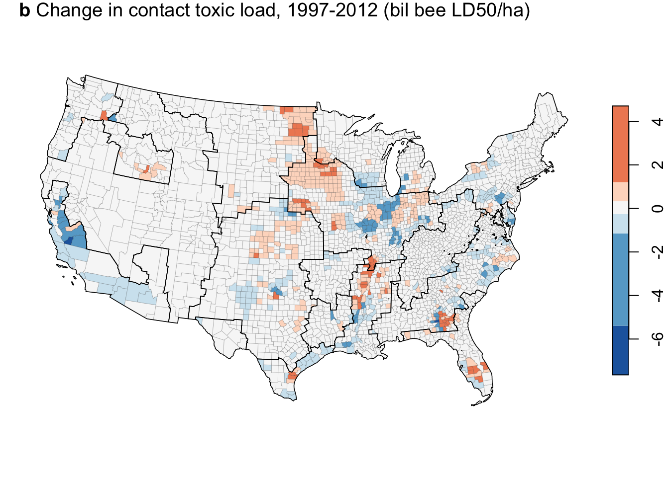
#title("b) Change in contact toxic load, 1997-2012 (bil bee LD50/ha)", adj = 0)Oral toxic load 2012
my_pal <- brewer.pal(n = 6, name = "BuPu")
or_tox_ha_12 <- filter(cnty_sf_join, var=="or_tox_ha" & is.finite(value))

plot(or_tox_ha_12["value"],
     pal = my_pal,
     breaks = "jenks",
     nbreaks = 6,
     main = "",
     lwd = 0.1,
     key.width = .1,
     reset=FALSE)
Warning in classInt::classIntervals(na.omit(values), min(nbreaks, n.unq), :
N is large, and some styles will run very slowly; sampling imposedUse "fisher" instead of "jenks" for larger data setsplot(regions,
main = "",
pal = clear_pal,
lwd = 0.8,
key.pos = NULL,
add=T)
title(expression(paste(bold("c"), " Oral toxic load 2012 (bil bee LD50/ha)")), adj = 0)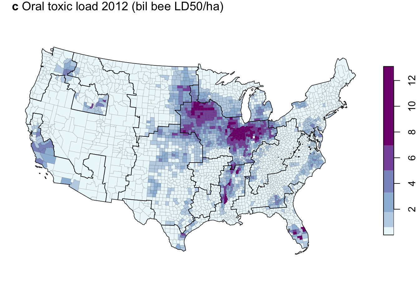
#title("c) Oral toxic load 2012 (bil bee LD50/ha)", adj = 0)Change in oral toxic load 1997-2012
my_pal <- c("#D1E5F0", "#F7F7F7", "#FDDBC7", "#F4A582", "#D6604D", "#B2182B", "#67001F")
or_tox_ha_12 <- filter(cnty_sf_join, var=="or_tox_ha" & is.finite(chg))

int <- classIntervals(or_tox_ha_12$chg, n = 6, style = "jenks")
Warning in classIntervals(or_tox_ha_12$chg, n = 6, style = "jenks"): N is
large, and some styles will run very slowly; sampling imposedUse "fisher" instead of "jenks" for larger data setsbrks <- sort(append(int$brks, -.55))
plot(or_tox_ha_12["chg"],
pal = my_pal,
breaks = brks,
nbreaks = 7,
key.width = 0.1,
lwd = 0.1,
main = "",
reset=FALSE)
plot(regions,
main = "",
pal = clear_pal,
lwd = 0.8,
key.pos = NULL,
add=T)
title(expression(paste(bold("d"), " Change in oral toxic load, 1997-2012 (bil bee LD50/ha)")), adj = 0)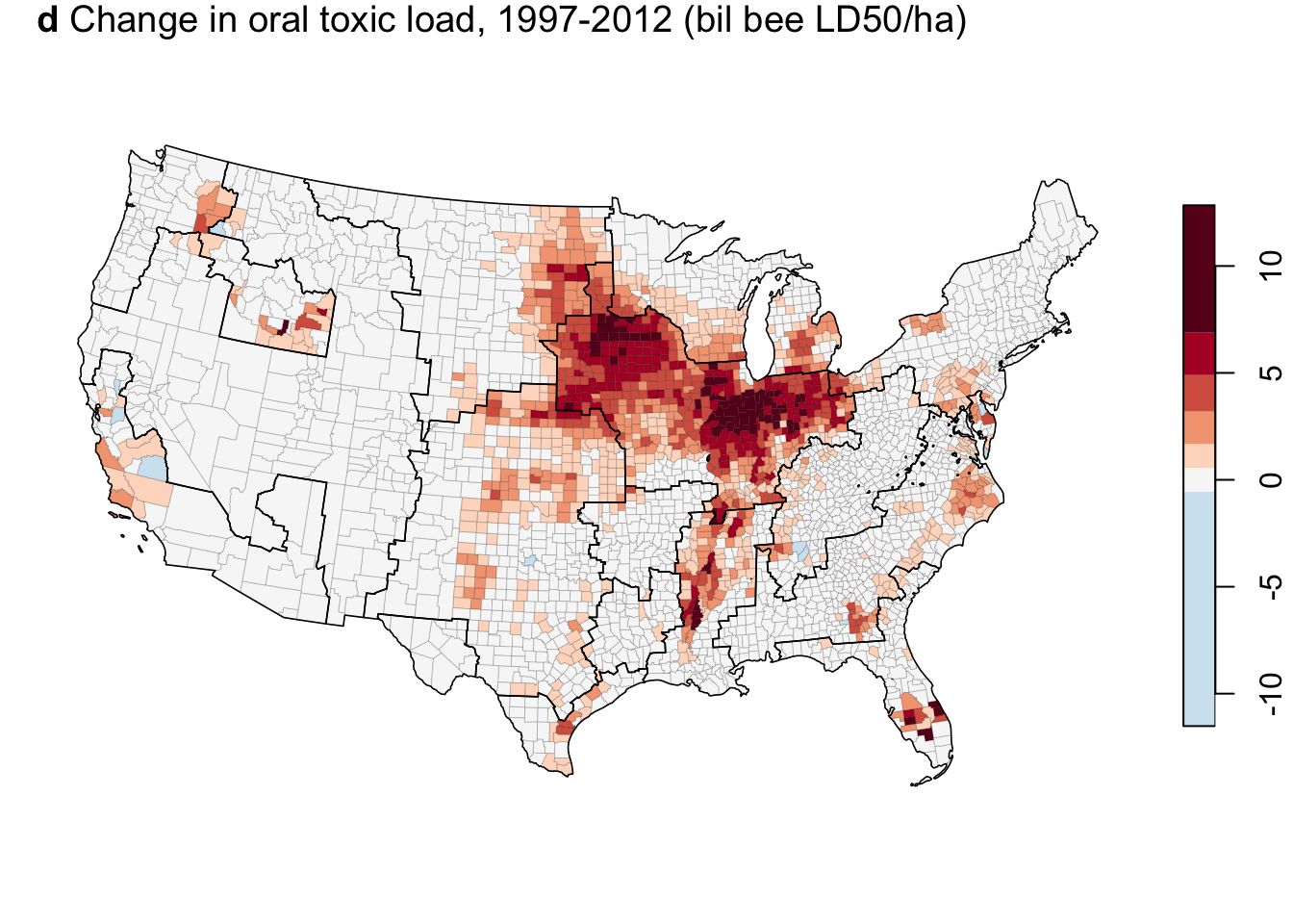
#title("d) Change in oral toxic load, 1997-2012 (bil bee LD50/ha)", adj = 0)Ag resource regions
plot(regions,
     main = "",
     lwd = 0.8,
     key.width = lcm(5.2))
plot(cnty_sf_join$geometry,
     lwd = 0.01,
     border = "black",
     add=T)
title("Agricultural resource regions", adj = 0)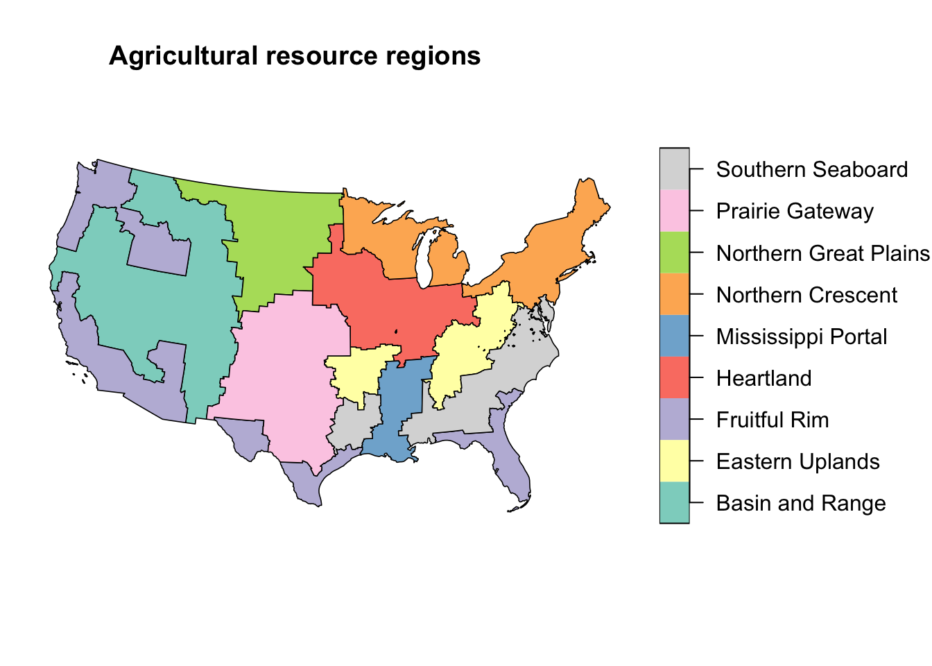
Session information
sessionInfo()R version 3.6.1 (2019-07-05)
Platform: x86_64-apple-darwin15.6.0 (64-bit)
Running under: macOS High Sierra 10.13.6
Matrix products: default
BLAS: /Library/Frameworks/R.framework/Versions/3.6/Resources/lib/libRblas.0.dylib
LAPACK: /Library/Frameworks/R.framework/Versions/3.6/Resources/lib/libRlapack.dylib
locale:
[1] en_US.UTF-8/en_US.UTF-8/en_US.UTF-8/C/en_US.UTF-8/en_US.UTF-8
attached base packages:
[1] stats graphics grDevices utils datasets methods base
other attached packages:
[1] classInt_0.3-3 RColorBrewer_1.1-2 tigris_0.8.2
[4] sf_0.7-6 sp_1.3-1 forcats_0.4.0
[7] stringr_1.4.0 dplyr_0.8.3 purrr_0.3.2
[10] readr_1.3.1 tidyr_0.8.3 tibble_2.1.3
[13] ggplot2_3.2.0 tidyverse_1.2.1
loaded via a namespace (and not attached):
[1] tidyselect_0.2.5 xfun_0.8 haven_2.1.1
[4] lattice_0.20-38 colorspace_1.4-1 generics_0.0.2
[7] vctrs_0.2.0 htmltools_0.3.6 yaml_2.2.0
[10] rlang_0.4.0 e1071_1.7-2 pillar_1.4.2
[13] foreign_0.8-71 glue_1.3.1 withr_2.1.2
[16] DBI_1.0.0 rappdirs_0.3.1 uuid_0.1-2
[19] modelr_0.1.4 readxl_1.3.1 munsell_0.5.0
[22] gtable_0.3.0 cellranger_1.1.0 rvest_0.3.4
[25] evaluate_0.14 labeling_0.3 knitr_1.23
[28] maptools_0.9-5 curl_3.3 class_7.3-15
[31] broom_0.5.2 Rcpp_1.0.1 KernSmooth_2.23-15
[34] scales_1.0.0 backports_1.1.4 jsonlite_1.6
[37] hms_0.5.0 digest_0.6.20 stringi_1.4.3
[40] grid_3.6.1 rgdal_1.4-4 cli_1.1.0
[43] tools_3.6.1 magrittr_1.5 lazyeval_0.2.2
[46] crayon_1.3.4 pkgconfig_2.0.2 zeallot_0.1.0
[49] xml2_1.2.0 lubridate_1.7.4 assertthat_0.2.1
[52] rmarkdown_1.14 httr_1.4.0 rstudioapi_0.10
[55] R6_2.4.0 units_0.6-3 nlme_3.1-140
[58] compiler_3.6.1 This R Markdown site was created with workflowr