Validation - pesticide use values

Purpose

This code compares pesticide use estimates across independent datasets for major crops (corn, soy, wheat, cotton, rice). The comparisons include:

total amount applied (kg)
application rate (kg/ha) calculated by dividing the USDA total kg by our new estimate of crop area (ha)
application rate (kg/ha) derived indirectly by multiplying the USDA average application rate on treated hectares by the percent of area treated

Libraries & functions

library(tidyverse)
library(readxl)
library(dplyr)
library(ggplot2)
library(gridExtra)

Load and join data

## Key relating USDA and USGS pesticide names
pesticide_names <- read_excel("../keys/usda_usgs_pesticide_names.xlsx")

# check for duplicates
usgs_pesticide_dups <- pesticide_names %>%
  group_by(usgs_cmpd) %>%
  mutate(n = n()) %>%
  filter(Match_status != "missing")
# some USGS names correspond to > 1 USDA name

usda_pesticide_dups <- pesticide_names %>%
  group_by(usda_cmpd) %>%
  mutate(n = n())
# no true duplicates in USDA names (some extra spaces, etc.)

## USGS pesticide estimates
usgs <- read.csv("../output_big/bee_tox_index_state_yr_cmpd_20200609.csv") %>%
  mutate(crop = toupper(crop)) 

## USDA pesticide estimates
usda <- read.csv("../output_big/nass_survey/qs.environment.pest.st.app.rate.usgs_20200528.csv")

# Join USDA estimates and name key
usda_key <- left_join(usda, pesticide_names, by = c("DOMAINCAT_DESC" = "usda_cmpd"))%>%
  mutate(kg_usda = lb*0.453592)

## Sum kg_usda values for data with repeated USGS cmpd, year, crop, and state
# aggregate cases in which multiple USDA AIs correspond to one USGS AI
usda_agg <- usda_key %>%
  group_by(YEAR, STATE_ALPHA, usgs_cmpd, COMMODITY_DESC, CLASS_DESC, usda_category) %>%
  summarise(n_usda = length(kg_usda),
            kg_usda = sum(kg_usda, na.rm = TRUE),
            kg_ha_yr_ave = sum(kg_ha_yr_ave, na.rm = TRUE),
            perc_trt_ave = sum(perc_trt_ave, na.rm = TRUE)) %>%
  mutate(perc_trt_alt = ifelse(perc_trt_ave <= 100, perc_trt_ave, 100)) %>%  # create new % trt column bounded at 100%
  rename(CROP = COMMODITY_DESC) %>%
  ungroup()

## `summarise()` has grouped output by 'YEAR', 'STATE_ALPHA', 'usgs_cmpd', 'COMMODITY_DESC', 'CLASS_DESC'. You can override using the `.groups` argument.

usda_agg <- usda_agg[!is.na(usda_agg$usgs_cmpd), ] # remove rows without USGS compound

# aggregate cases in which multiple values for a given crop-state-year-AI combo (only occurs in wheat)
# this is imperfect b/c ideally the averages would be weighted by acreage
usda_agg_other <- filter(usda_agg, CROP != "WHEAT") %>%
  select(-CLASS_DESC) %>%
  mutate(n_crop = 1) %>%
  select(YEAR, STATE_ALPHA, usgs_cmpd, CROP, usda_category, n_usda, n_crop, kg_usda, kg_ha_yr_ave, perc_trt_ave, perc_trt_alt)

usda_agg_wheat <- filter(usda_agg, CROP == "WHEAT") %>%
  group_by(YEAR, STATE_ALPHA, usgs_cmpd, CROP, usda_category) %>%
  summarise(n_usda = sum(n_usda),
            n_crop = length(kg_usda),
            kg_usda = sum(kg_usda, na.rm = TRUE),
            kg_ha_yr_ave = mean(kg_ha_yr_ave, na.rm = TRUE),
            perc_trt_ave = mean(perc_trt_ave, na.rm = TRUE),
            perc_trt_alt = mean(perc_trt_alt, na.rm = TRUE)) %>%
  ungroup()

## `summarise()` has grouped output by 'YEAR', 'STATE_ALPHA', 'usgs_cmpd', 'CROP'. You can override using the `.groups` argument.

usda_full <- bind_rows(usda_agg_other, usda_agg_wheat)

## Join aggregated USDA estimates and USGS estimate
joined <- inner_join(usda_full, usgs,
                               by=c("usgs_cmpd"="cmpd_usgs",
                                    "STATE_ALPHA"="STATE_ALPHA",
                                    "YEAR"="Year",
                                    "CROP"="crop"))%>%
  mutate(kg_ha_usda = kg_usda/ha,
         kg_ha2_usda = (kg_ha_yr_ave),
         kg_thou_usda = kg_usda/10^3,
         kg_thou_usgs = kg_app/10^3)

joined[joined == 0] <- NA  # restore NA values

Subset and clean data

# Select for desired years and crops
crops <- c("CORN", "SOYBEANS", "WHEAT", "COTTON", "RICE")
target <- c(1997:2017)
category <- c("Insecticide", "Herbicide", "Fungicide")

# Prep dataset
clean <- joined %>%
  filter(CROP %in% crops,
         YEAR %in% target,
         usda_category %in% category)%>%
  mutate(kg_ha_usgs = kg_ha)%>%
  select(kg_app,
         kg_usda,
         kg_thou_usda,
         kg_thou_usgs,
         kg_ha_usda,
         kg_ha2_usda,
         kg_ha_usgs,
         CROP,
         usda_category,
         STATE_ALPHA,
         YEAR,
         usgs_cmpd,
         n_usda,
         n_crop,
         perc_trt_alt,
         ha)

# create groups for percent treated
perc_grp_tags <- c("10","20", "30", "40", "50", "60", "70", "80","90", "90+") 

diff <- clean %>%
  mutate(kg_diff = kg_app - kg_usda,
         kg_ha_diff1 = kg_ha_usgs - kg_ha_usda,
         kg_ha_diff2 = kg_ha_usgs - kg_ha2_usda,
         RE_kg = (kg_diff/((kg_app + kg_usda)/2))*100,
         RE_kg_ha_diff1 = (kg_ha_diff1/((kg_ha_usgs + kg_ha_usda)/2))*100,
         RE_kg_ha_diff2 = (kg_ha_diff2/((kg_ha_usgs + kg_ha2_usda)/2))*100) %>%
  mutate(perc_grp = case_when(
    perc_trt_alt < 10 ~ perc_grp_tags[1],
    perc_trt_alt >= 10 & perc_trt_alt < 20 ~ perc_grp_tags[2],
    perc_trt_alt >= 20 & perc_trt_alt < 30 ~ perc_grp_tags[3],
    perc_trt_alt >= 30 & perc_trt_alt < 40 ~ perc_grp_tags[4],
    perc_trt_alt >= 40 & perc_trt_alt < 50 ~ perc_grp_tags[5],
    perc_trt_alt >= 50 & perc_trt_alt < 60 ~ perc_grp_tags[6],
    perc_trt_alt >= 60 & perc_trt_alt < 70 ~ perc_grp_tags[7],
    perc_trt_alt >= 70 & perc_trt_alt < 80 ~ perc_grp_tags[8],
    perc_trt_alt >= 80 & perc_trt_alt < 90 ~ perc_grp_tags[9],
    perc_trt_alt >= 90 ~ perc_grp_tags[10]
  ))

Visualize patterns

Difference by area treated

ggplot(data = drop_na(diff, perc_trt_alt), mapping = aes(x = perc_grp, y = RE_kg)) + 
  geom_jitter(color = "darkturquoise", alpha=0.1) +
  geom_boxplot(fill="ivory3", color="black", alpha=0.3) + 
  geom_hline(yintercept = 0, lty = 2) +
  ggtitle('a) kg applied') +
  labs(x = '% crop area treated (USDA)',
       y = 'Relative difference (%)') +
  guides(color=FALSE) +
  theme_minimal(base_size = 18)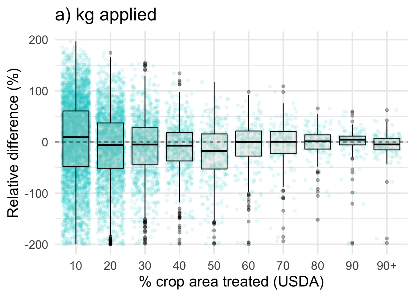

ggplot(data = drop_na(diff, perc_trt_alt), mapping = aes(x = perc_grp, y = RE_kg_ha_diff1)) + 
  geom_jitter(color = "mediumorchid1", alpha=0.2) +
  geom_boxplot(fill="ivory3", color="black", alpha=0.2) + 
  geom_hline(yintercept = 0, lty = 2) +
  ggtitle('b) kg/ha - Method 1') +
  labs(x = '% crop area treated (USDA)',
       y = 'Relative difference (%)') +
  guides(color=FALSE) +
  theme_minimal(base_size = 18)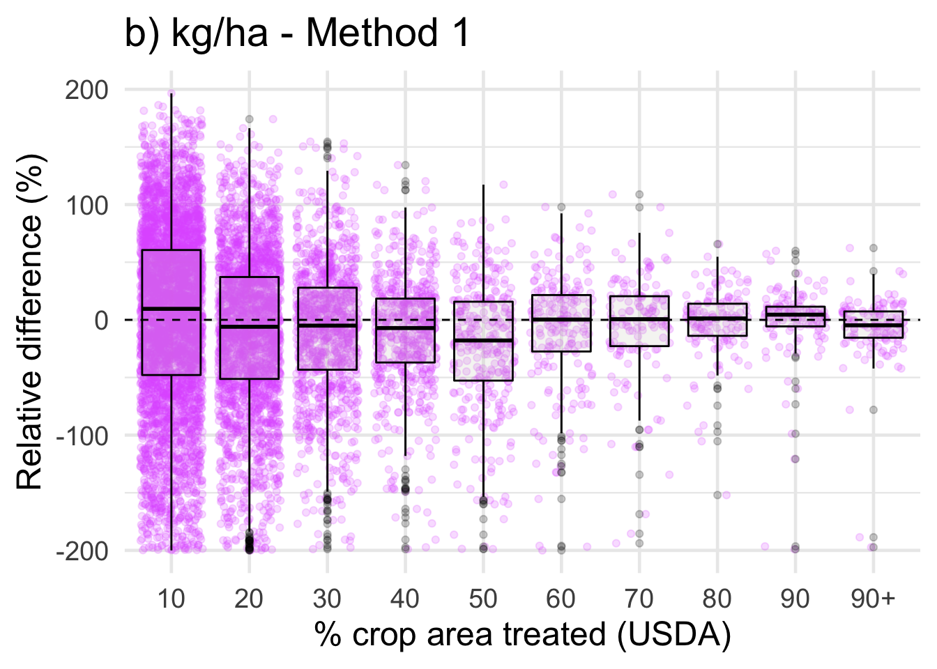

ggplot(data = drop_na(diff, perc_trt_alt), mapping = aes(x = perc_grp, y = RE_kg_ha_diff2)) + 
  geom_jitter(color = "coral1", alpha=0.1) +
  geom_boxplot(fill="ivory3", color="black", alpha=0.3) + 
  geom_hline(yintercept = 0, lty = 2) +
  ggtitle('c) kg/ha - Method 2') +
  labs(x = '% crop area treated (USDA)',
       y = 'Relative difference (%)') +
  guides(color=FALSE) +
  theme_minimal(base_size = 18)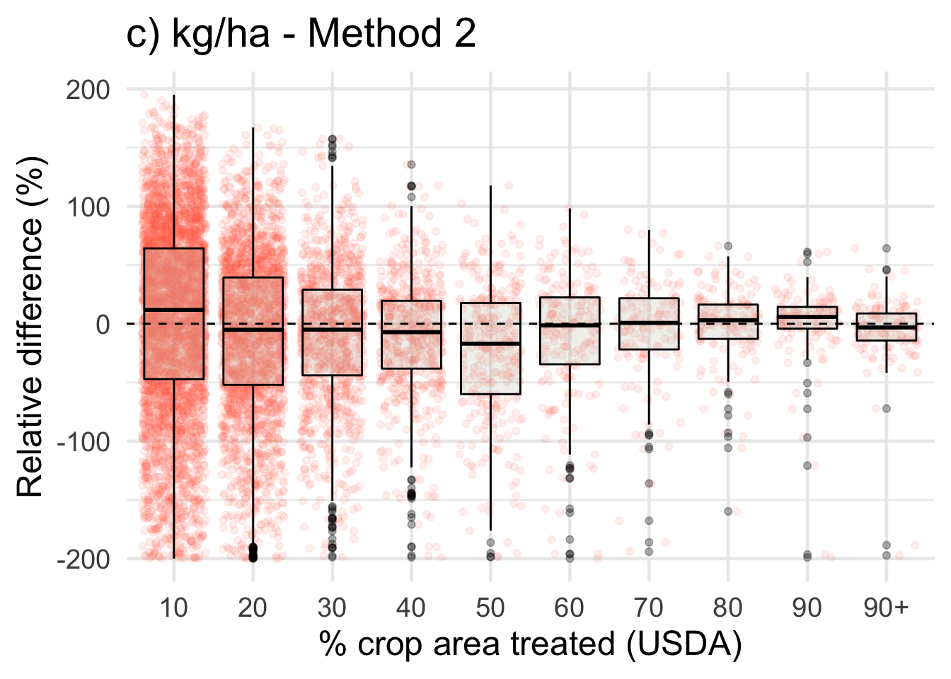

Save figure for publication

require(gridExtra)

a <- ggplot(data = drop_na(diff, perc_trt_alt), mapping = aes(x = perc_grp, y = RE_kg)) + 
  geom_jitter(color = "darkturquoise", alpha=0.1) +
  geom_boxplot(fill="ivory3", color="black", alpha=0.3) + 
  geom_hline(yintercept = 0, lty = 2) +
  ggtitle('a) kg applied') +
  labs(x = '% crop area treated (USDA)',
       y = 'Relative difference (%)') +
  guides(color="none") +
  theme_minimal(base_size = 18)

b <- ggplot(data = drop_na(diff, perc_trt_alt), mapping = aes(x = perc_grp, y = RE_kg_ha_diff1)) + 
  geom_jitter(color = "mediumorchid1", alpha=0.2) +
  geom_boxplot(fill="ivory3", color="black", alpha=0.2) + 
  geom_hline(yintercept = 0, lty = 2) +
  ggtitle('b) kg/ha - Method 1') +
  labs(x = '% crop area treated (USDA)',
       y = 'Relative difference (%)') +
  guides(color="none") +
  theme_minimal(base_size = 18)

c <- ggplot(data = drop_na(diff, perc_trt_alt), mapping = aes(x = perc_grp, y = RE_kg_ha_diff2)) + 
  geom_jitter(color = "coral1", alpha=0.1) +
  geom_boxplot(fill="ivory3", color="black", alpha=0.3) + 
  geom_hline(yintercept = 0, lty = 2) +
  ggtitle('c) kg/ha - Method 2') +
  labs(x = '% crop area treated (USDA)',
       y = 'Relative difference (%)') +
  guides(color="none") +
  theme_minimal(base_size = 18)

ggsave("../docs/validation_values_files/figure-html/fig3.pdf", 
       arrangeGrob(a,b,c),
       width = 3,
       height = 9,
       scale = 1.8)

Difference by area treated and crop

ggplot(data = drop_na(diff, perc_trt_alt), mapping = aes(x = perc_grp, y = RE_kg)) + 
  geom_jitter(aes(color = CROP), alpha=0.2) +
  geom_boxplot(fill="bisque", color="black", alpha=0.3) + 
  geom_hline(yintercept = 0, lty = 2) +
  ggtitle('kg applied') +
  labs(x = '% crop area treated (USDA)',
       y = 'Relative difference (%)') +
  facet_grid(~ CROP) +
  guides(color=FALSE) +
  theme_minimal()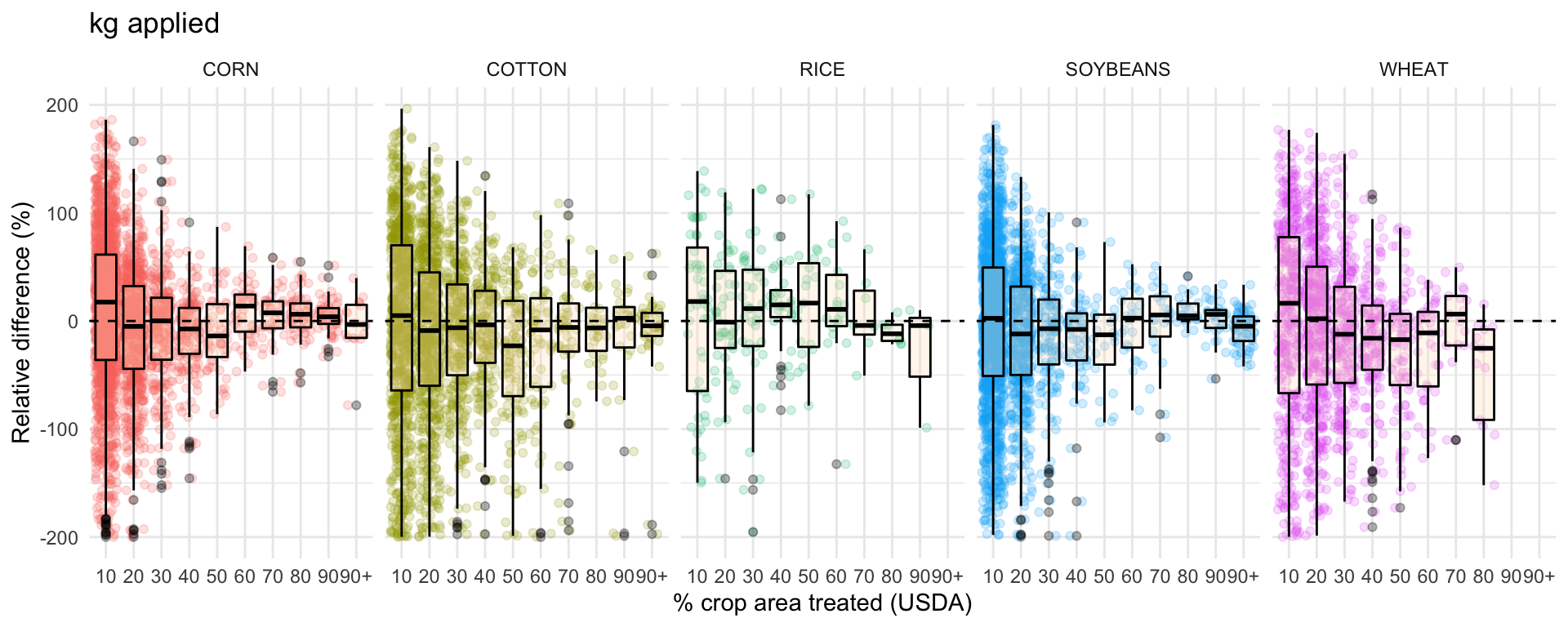

ggplot(data = drop_na(diff, perc_trt_alt), mapping = aes(x = perc_grp, y = RE_kg_ha_diff1)) + 
  geom_jitter(aes(color = CROP), alpha=0.2) +
  geom_boxplot(fill="bisque", color="black", alpha=0.3) + 
  geom_hline(yintercept = 0, lty = 2) +
  ggtitle('kg/ha - Method 1') +
  labs(x = '% crop area treated (USDA)',
       y = 'Relative difference (%)') +
  facet_grid(~ CROP) +
  guides(color=FALSE) +
  theme_minimal()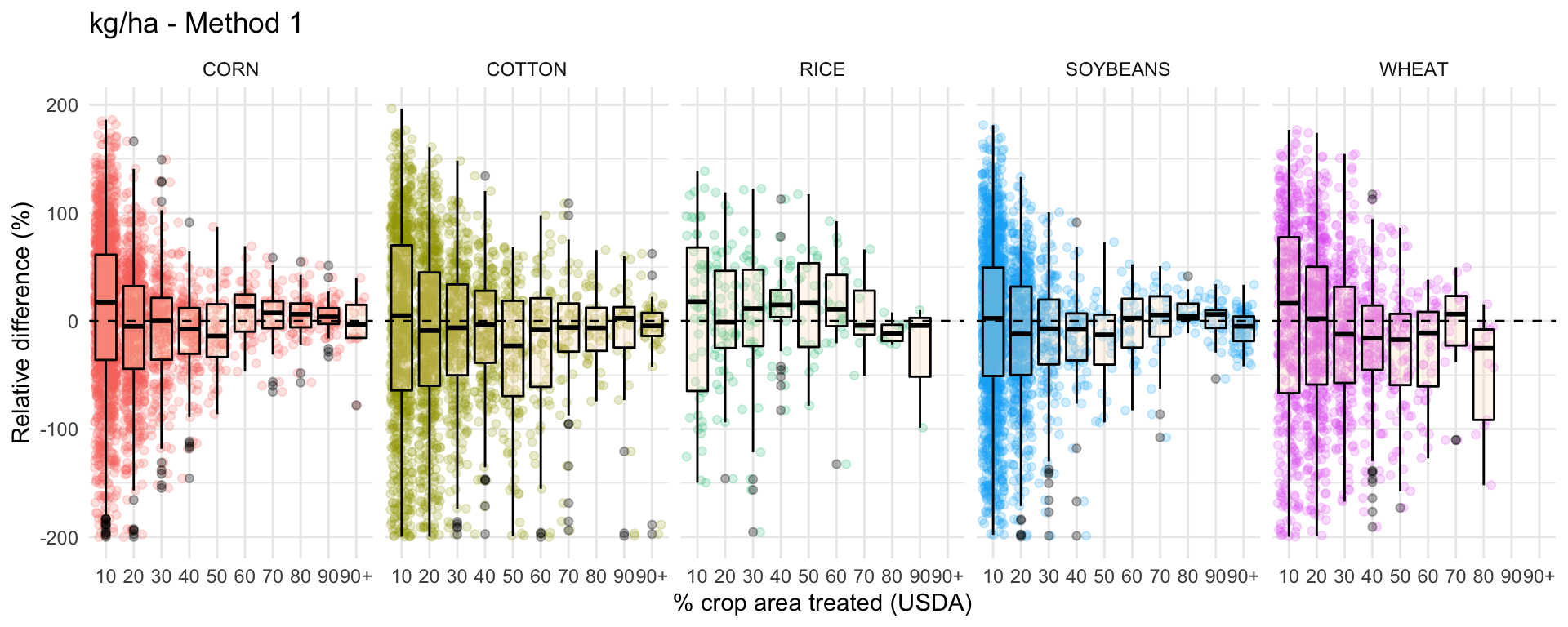

ggplot(data = drop_na(diff, perc_trt_alt), mapping = aes(x = perc_grp, y = RE_kg_ha_diff2)) + 
  geom_jitter(aes(color = CROP), alpha=0.2) +
  geom_boxplot(fill="bisque", color="black", alpha=0.3) + 
  geom_hline(yintercept = 0, lty = 2) +
  ggtitle('kg/ha - Method 2') +
  labs(x = '% crop area treated (USDA)',
       y = 'Relative difference (%)') +
  facet_grid(~ CROP) +
  guides(color=FALSE) +
  theme_minimal()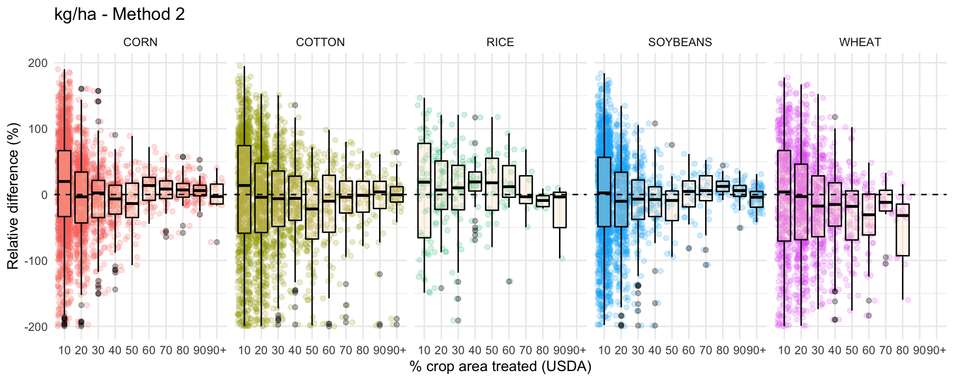

Restructure for additional plotting

# Restructure corrected estimates data for plots
# rename USGS data columns according to the method of analysis their values will be used in

names(clean)[names(clean)=="kg_thou_usgs"] <- "kg_thou"
names(clean)[names(clean)=="kg_ha_usgs"] <- "method_1"

# create data set with only USGS values
# duplicate and rename method 1 values so that they can be used for method 2 analysis
# turn to long form

usgs_cl <- clean %>%
  select(kg_thou,
         method_1,
         CROP,
         STATE_ALPHA,
         YEAR,
         usgs_cmpd,
         usda_category)%>%
  mutate(method_2 = method_1) %>%
  gather("kg_thou","method_1","method_2",
          key = "method",
          value = "usgs")

# create data set with only USDA values
# turn to long form

usda_cl <- clean %>%
  select(kg_thou_usda,
         kg_ha_usda,
         kg_ha2_usda,
         STATE_ALPHA,
         YEAR,
         usgs_cmpd,
         CROP,
         usda_category) %>%
  rename(kg_thou = kg_thou_usda,
         method_1 = kg_ha_usda,
         method_2 = kg_ha2_usda) %>%
  gather("kg_thou", "method_1","method_2",
         key = "method",
         value = "usda")

# join altered usgs and usda data with single methods column;
# unite methods and usda category to allow facet wrap to be used

graph_data <- full_join(usda_cl, usgs_cl,
                           by=c("CROP",
                                "STATE_ALPHA",
                                "YEAR",
                                "method",
                                "usgs_cmpd",
                                "usda_category"))%>%
  unite("methods", c("method", "usda_category"), remove = FALSE) %>%
  mutate(diff = usgs-usda,
         RE = (diff/((usda+usgs)/2)*100))

graph_data$method_pretty <- recode(graph_data$methods,
                             kg_thou_Fungicide = "Fungicides (1000 kg)",
                             kg_thou_Insecticide = "Insecticides (1000 kg)",
                             kg_thou_Herbicide = "Herbicides (1000 kg)",
                             method_1_Fungicide = "Fungicides (kg/ha - Method 1)",
                             method_1_Herbicide = "Herbicides (kg/ha - Method 1)",
                             method_1_Insecticide = "Insecticides (kg/ha - Method 1)",
                             method_2_Fungicide = "Fungicides (kg/ha - Method 2)",
                             method_2_Herbicide = "Herbicides (kg/ha - Method 2)",
                             method_2_Insecticide = "Insecticides (kg/ha - Method 2)")

# export comparison dataset for low values
write.csv(graph_data, "../output_big/validation_low_estimate.csv", row.names = FALSE)

Plot estimates against each other

# plot by methods of analysis and USDA category;
# create invisible matching points so that each graph x-axis=y-axis

ggplot(graph_data, aes(x=usda, y=usgs, color=CROP))+
  geom_point(mapping=aes(x=usda,
                         y=usgs),
             alpha = 0.4)+
  geom_point(mapping=aes(x=usgs,
                         y=usda),
             alpha=0)+
  geom_abline(linetype = 2)+
  facet_wrap("methods", scales="free") +
  theme_classic() +
  xlab("USDA estimate") +
  ylab("USGS-based estimate")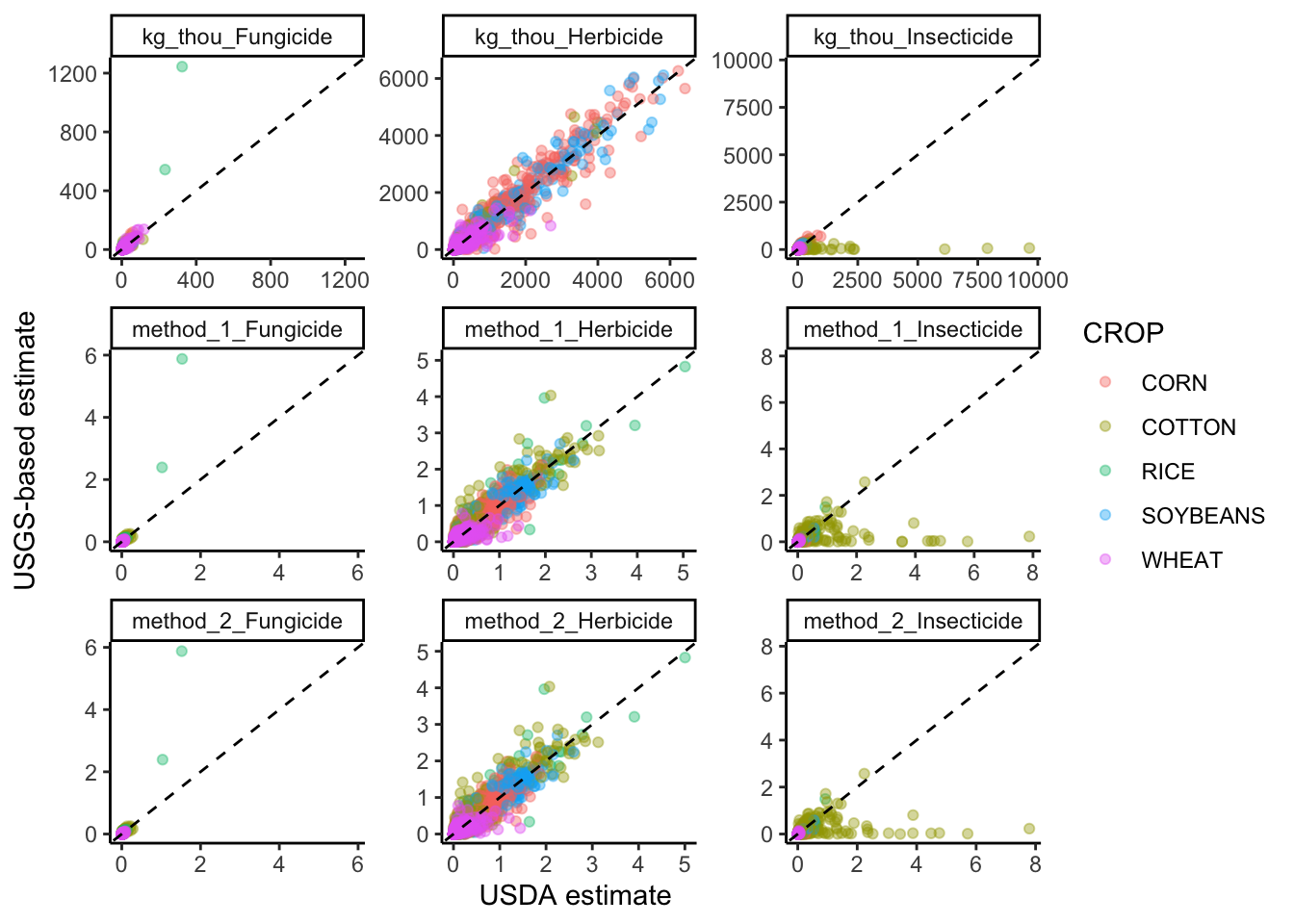

# remove outliers
ggplot(filter(graph_data, 
              !(CROP == "COTTON" & usgs_cmpd == "MALATHION")
              & !(CROP == "RICE" & usgs_cmpd == "COPPERSULFATE")), 
       aes(x=usda, y=usgs, color=CROP))+
  geom_point(mapping=aes(x=usda,
                         y=usgs),
             alpha = 0.4)+
  geom_point(mapping=aes(x=usgs,
                         y=usda),
             alpha=0)+
  geom_abline(linetype = 2)+
  facet_wrap("method_pretty", scales="free") +
  xlab("USDA estimate") +
  ylab("USGS-based estimate") +
  theme_classic() +
  theme(strip.background = element_blank())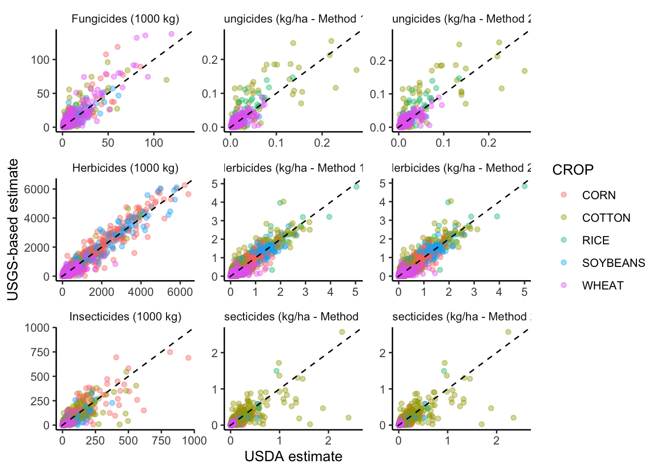

Save figure for publication

# open file
pdf(file = "../docs/validation_values_files/figure-html/fig2.pdf",   # The directory you want to save the file in
    width = 8, # The width of the plot in inches
    height = 6) # The height of the plot in inches

# remove outliers
ggplot(filter(graph_data, 
              !(CROP == "COTTON" & usgs_cmpd == "MALATHION")
              & !(CROP == "RICE" & usgs_cmpd == "COPPERSULFATE")), 
       aes(x=usda, y=usgs, color=CROP))+
  geom_point(mapping=aes(x=usda,
                         y=usgs),
             alpha = 0.4)+
  geom_point(mapping=aes(x=usgs,
                         y=usda),
             alpha=0)+
  geom_abline(linetype = 2)+
  facet_wrap("method_pretty", scales="free") +
  xlab("USDA estimate") +
  ylab("USGS-based estimate") +
  theme_classic() +
  theme(strip.background = element_blank()) 

# Run dev.off() to create the file!
dev.off()

## quartz_off_screen 
##                 2

Boxplot of RE by class

# plot by methods of analysis and USDA category;
# create invisible matching points so that each graph x-axis=y-axis

ggplot(graph_data, aes(x=method, y=RE, color=usda_category))+
  geom_boxplot() +
  geom_hline(yintercept = 0, linetype = 2) +
  #facet_wrap("method", scales="free") +
  theme_classic() +
  xlab("") +
  ylab("Relative difference (%)")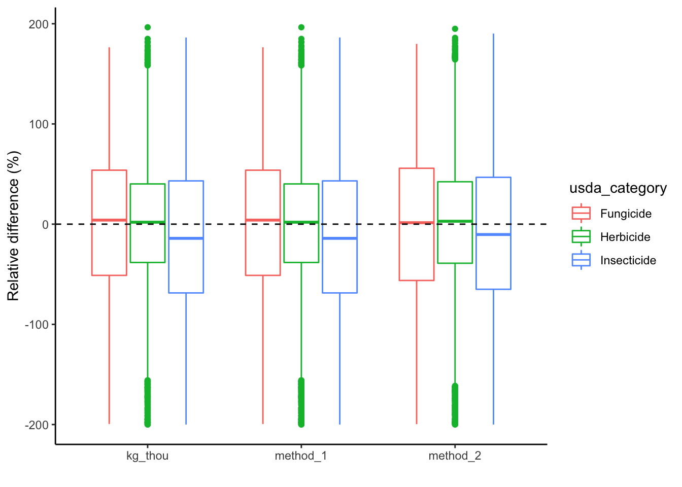

Boxplot of RE by crop + class

# plot by methods of analysis and USDA category;
# create invisible matching points so that each graph x-axis=y-axis

ggplot(graph_data, aes(x=CROP, y=RE, color=CROP))+
  geom_boxplot() +
  geom_hline(yintercept = 0, linetype = 2) +
  facet_wrap("methods", scales="free") +
  theme_classic() +
  xlab("") +
  ylab("Relative difference (%)")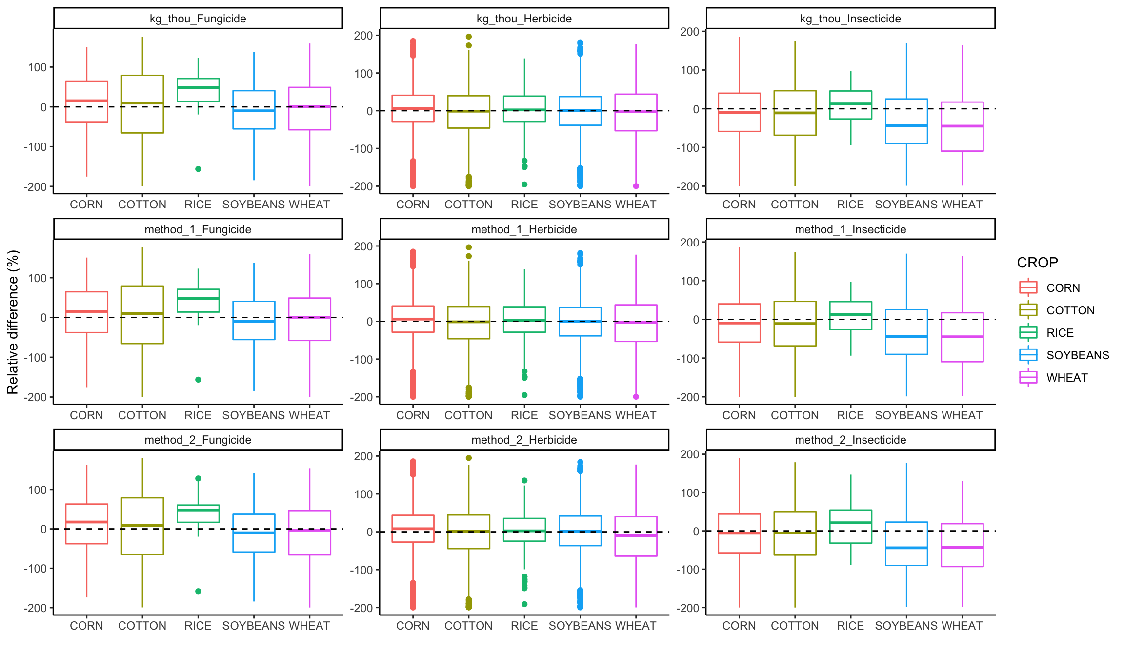

Boxplot of RE by year

# plot by methods of analysis and USDA category;
# create invisible matching points so that each graph x-axis=y-axis

ggplot(graph_data, aes(x=as.factor(YEAR), y=RE))+
  geom_boxplot() +
  geom_hline(yintercept = 0, linetype = 2) +
  facet_wrap("CROP", scales="free") +
  theme_classic() +
  xlab("") +
  ylab("Relative difference (%)")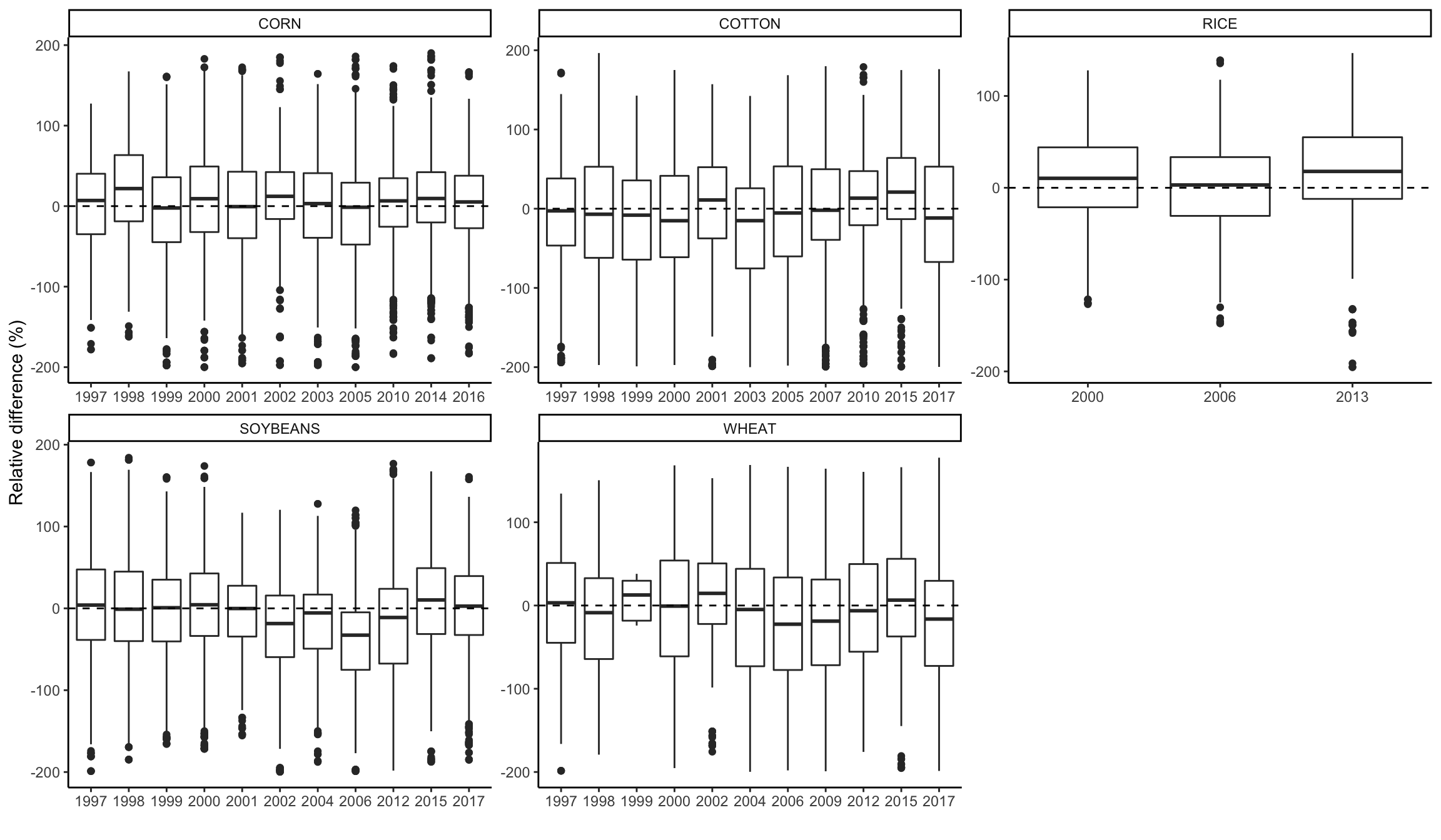

Example trends comparison

# e.g. for glyphosate
# plot by methods of analysis and USDA category;
# create invisible matching points so that each graph x-axis=y-axis

filtered_data <- graph_data %>%
  filter(methods == "method_2_Herbicide",
         usgs_cmpd == "GLYPHOSATE",
         CROP == "SOYBEANS",
         !STATE_ALPHA %in% c("MD","DE")) %>%
  select(-diff, -RE) %>%
  pivot_longer(cols = usda:usgs,
               names_to = "source",
               values_to = "kg_ha")

ggplot(filtered_data, aes(x = YEAR, y = kg_ha, group = source)) +
  geom_line(aes(linetype = source)) +
  facet_wrap("STATE_ALPHA", scales = "free_y") +
  theme_classic() +
  xlab("") +
  ylab("Application rate (kg/ha)")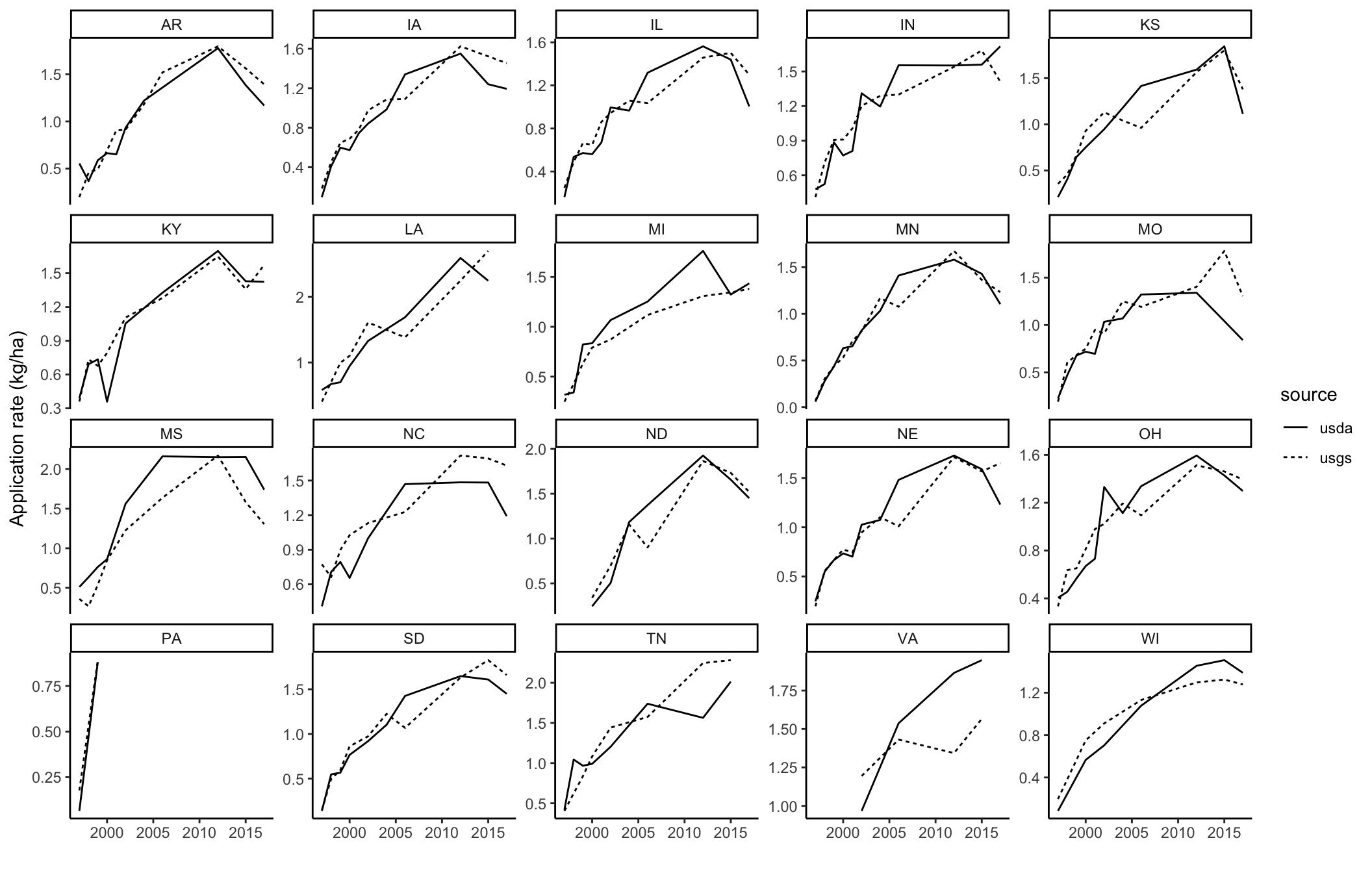

Calculate summary statistics

By category

stats <- graph_data %>%
  drop_na() %>%
  group_by(usda_category, method) %>%
  summarise(n = n(),
            med_RE = round(median(RE, na.rm=T), digits = 1),
            iqr_25 = round(quantile(RE, .25, na.rm=T), digits = 1),
            iqr_75 = round(quantile(RE, .75, na.rm=T), digits = 1),
            wilcox_p = (wilcox.test(RE, mu = 0, alternative = "two.sided", conf.int=T, conf.level = 0.05))$p.value,
            rank_corr = round(cor(usgs, usda, method = "spearman", use = "pairwise.complete.obs"), digits = 2),
            corr = round(cor(usgs, usda, method = "pearson", use = "pairwise.complete.obs"), digits = 2)
            )

## `summarise()` has grouped output by 'usda_category'. You can override using the `.groups` argument.

`%notin%` <- Negate(`%in%`)

out_removed <- filter(graph_data, 
                      !(CROP == "COTTON" & usgs_cmpd == "MALATHION"))

stats_out_removed <- out_removed %>%
  drop_na() %>%
  group_by(usda_category, method) %>%
  summarise(n = n(),
            med_RE = round(median(RE, na.rm=T), digits = 1),
            iqr_25 = round(quantile(RE, .25, na.rm=T), digits = 1),
            iqr_75 = round(quantile(RE, .75, na.rm=T), digits = 1),
            wilcox = (wilcox.test(RE, mu = 0, alternative = "two.sided"))$p.value,
            rank_corr = round(cor(usgs, usda, method = "spearman", use = "pairwise.complete.obs"), digits = 2),
            corr = round(cor(usgs, usda, method = "pearson", use = "pairwise.complete.obs"), digits = 2))

## `summarise()` has grouped output by 'usda_category'. You can override using the `.groups` argument.

stats_total <- graph_data %>%
  group_by(method) %>%
  drop_na() %>%
  summarise(n = n(),
            med_RE = round(median(RE, na.rm=T), digits = 1),
            iqr_25 = round(quantile(RE, .25, na.rm=T), digits = 1),
            iqr_75 = round(quantile(RE, .75, na.rm=T), digits = 1),
            wilcox = (wilcox.test(RE, mu = 0, alternative = "two.sided"))$p.value,
            rank_corr = round(cor(usgs, usda, method = "spearman", use = "pairwise.complete.obs"), digits = 2),
            corr = round(cor(usgs, usda, method = "pearson", use = "pairwise.complete.obs"), digits = 2))

By compound

stats_cmpd <- graph_data %>%
  drop_na() %>%
  group_by(usgs_cmpd, usda_category, method) %>%
  summarise(med_RE = round(median(RE, na.rm=T), digits = 1),
            iqr_25 = round(quantile(RE, .25, na.rm=T), digits = 1),
            iqr_75 = round(quantile(RE, .75, na.rm=T), digits = 1),
            rank_corr = round(cor(usgs, usda, method = "spearman", use = "pairwise.complete.obs"), digits = 2),
            corr = round(cor(usgs, usda, method = "pearson", use = "pairwise.complete.obs"), digits = 2),
            n = n()) %>%
  filter(n > 10) %>%
  ungroup() %>%
  arrange(methods, usgs_cmpd)

By crop

stats_crop <- graph_data %>%
  drop_na() %>%
  group_by(CROP, usda_category, method) %>%
  summarise(med_RE = round(median(RE, na.rm=T), digits = 1),
            iqr_25 = round(quantile(RE, .25, na.rm=T), digits = 1),
            iqr_75 = round(quantile(RE, .75, na.rm=T), digits = 1),
            rank_corr = round(cor(usgs, usda, method = "spearman", use = "pairwise.complete.obs"), digits = 2),
            corr = round(cor(usgs, usda, method = "pearson", use = "pairwise.complete.obs"), digits = 2),
            n = n())

By year

stats_year <- graph_data %>%
  drop_na() %>%
  group_by(YEAR, usda_category, method) %>%
  summarise(med_RE = round(median(RE, na.rm=T), digits = 1),
            iqr_25 = round(quantile(RE, .25, na.rm=T), digits = 1),
            iqr_75 = round(quantile(RE, .75, na.rm=T), digits = 1),
            rank_corr = round(cor(usgs, usda, method = "spearman", use = "pairwise.complete.obs"), digits = 2),
            corr = round(cor(usgs, usda, method = "pearson", use = "pairwise.complete.obs"), digits = 2),
            n = n())

This R Markdown site was created with workflowr

Validation - pesticide use values

Paige Baisley + Maggie Douglas

Purpose

Libraries & functions

Load and join data

Subset and clean data

Visualize patterns

Difference by area treated

Save figure for publication

Difference by area treated and crop

Restructure for additional plotting

Plot estimates against each other

Save figure for publication

Boxplot of RE by class

Boxplot of RE by crop + class

Boxplot of RE by year

Example trends comparison

Calculate summary statistics

By category

By compound

By crop

By year