Sensitivity: Low vs. High USGS estimate
Maggie Douglas
Purpose
This code is intended to investigate the low vs. high pesticide data provided by USGS, in relation to independent pesticide estimates from USDA.
Load libraries + data
library(tidyverse)

## read in data comparing USGS to USDA values, for high and low estimate
high <- read.csv("../output_big/validation_high_estimate.csv") %>%
  mutate(type = "high")

low <- read.csv("../output_big/validation_low_estimate.csv") %>%
  mutate(type = "low")

# bind the two together
full <- rbind(high, low)

## read in full datasets
usgs_high <- read.csv("../output_big/bee_tox_index_state_yr_cmpd_high_20200609.csv") %>%
  select(-starts_with(c("ld50", "source"))) %>%
  rename_with(~ paste0(.x, "_h"), .cols = c("kg_app","kg_ha", "ha"))

usgs_low <- read.csv("../output_big/bee_tox_index_state_yr_cmpd_20200609.csv") %>%
    select(-starts_with(c("ld50", "source"))) %>%
    rename_with(~ paste0(.x, "_l"), .cols = c("kg_app","kg_ha", "ha"))

# join + create column for missing value in low estimate
usgs_full <- full_join(usgs_high, usgs_low, by = c("State_FIPS_code","State","Compound","Year","Units","crop",
                                                   "cmpd_usgs","STATE_ALPHA","cat","cat_grp","class","grp_source")) %>%
  mutate(low_missing = ifelse(is.na(kg_app_l), 1, 0))
Restructure data for plotting
high_val <- high %>%
  rename(usgs_high = usgs,
         RE_high = RE) %>%
  select(-diff, -method_pretty, -type)

joined <- low %>%
  rename(usgs_low = usgs,
         RE_low = RE) %>%
  select(-diff, -method_pretty, -type) %>%
  full_join(high_val, by = c("STATE_ALPHA", "YEAR", "usgs_cmpd", "CROP", "methods", "usda_category",
                             "method"))
Plot differences with USDA data
# plot by method of analysis and pesticide category
ggplot(full, aes(x = method, y = RE, fill = type))+
  geom_boxplot() +
  geom_hline(yintercept = 0, linetype = 2) +
  facet_grid("usda_category") +
  theme_classic() +
  coord_fixed(ratio = 0.005) +
  xlab("") +
  ylab("Relative difference to USDA (%)") +
  labs(fill = "USGS estimate")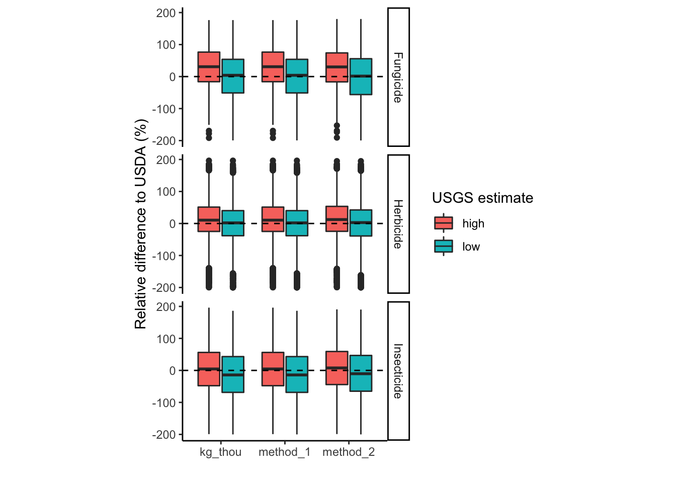
# plot by method of analysis for all AI combined
ggplot(full, aes(x = method, y = RE, fill = type))+
  geom_boxplot() +
  geom_hline(yintercept = 0, linetype = 2) +
  theme_classic() +
  xlab("") +
  ylab("Relative difference to USDA (%)") +
  labs(fill = "USGS estimate")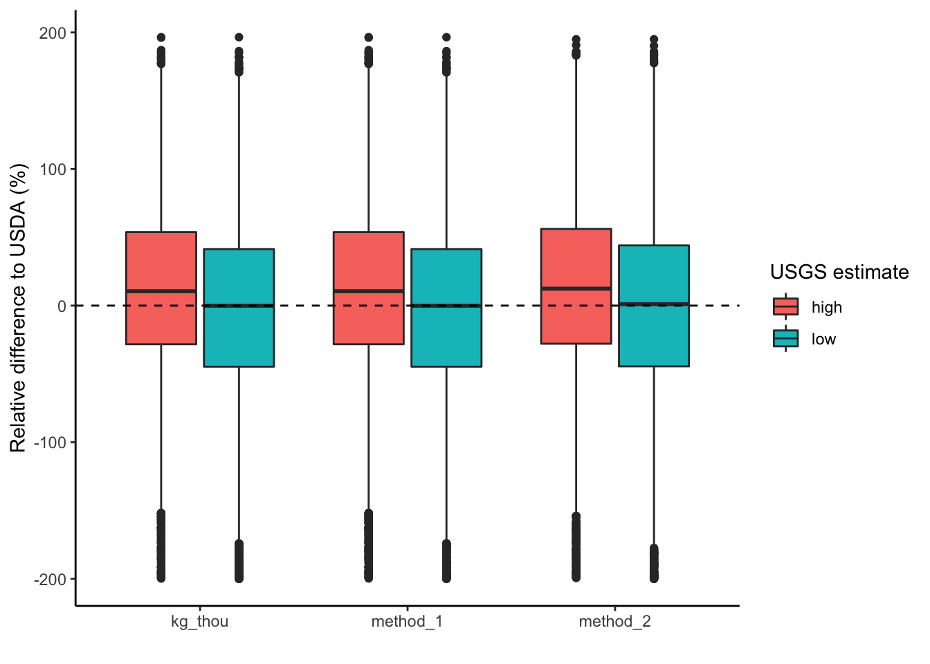
Investigate relationship between low and high estimate
# calculate correlation between the two estimates
cor(usgs_full$kg_ha_l, usgs_full$kg_ha_h, use = "pairwise.complete.obs")
## [1] 0.9522947# plot relationship
ggplot(usgs_full, aes(x = kg_ha_l, y = kg_ha_h)) +
geom_point(alpha = 0.3) +
theme_minimal(base_size = 18) +
xlab("USGS low (kg/ha)") +
ylab("USGS high (kg/ha)") +
geom_abline(slope = 1, intercept = 0, color = "red", linetype = 2) +
xlim(c(0,100)) +
ylim(c(0,100))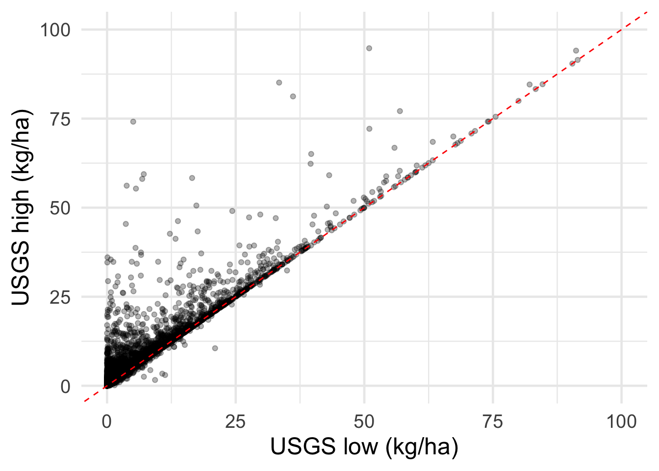
Summarize missing values in low dataset
summary(usgs_full$low_missing)## Min. 1st Qu. Median Mean 3rd Qu. Max.
## 0.00 0.00 0.00 0.17 0.00 1.00# summarize missing data by pesticide category
missing <- usgs_full %>%
group_by(cat) %>%
summarize(missing_n = sum(low_missing),
total_n = n(),
missing_perc = round(mean(low_missing), 2))
print.data.frame(missing)## cat missing_n total_n missing_perc
## 1 F 8319 69901 0.12
## 2 FUM 590 4094 0.14
## 3 H 32736 169828 0.19
## 4 I 17702 101215 0.17
## 5 O 237 2720 0.09
## 6 PGR 1365 10674 0.13# summarize missing data by pesticide crop
missing_crop <- usgs_full %>%
group_by(crop) %>%
summarize(missing_n = sum(low_missing),
total_n = n(),
missing_perc = round(mean(low_missing), 2))
print.data.frame(missing_crop)## crop missing_n total_n missing_perc
## 1 Alfalfa 5995 16141 0.37
## 2 Corn 13040 47467 0.27
## 3 Cotton 3839 24779 0.15
## 4 Orchards_and_grapes 4853 61567 0.08
## 5 Other_crops 6345 42153 0.15
## 6 Pasture_and_hay 4743 14379 0.33
## 7 Rice 370 4844 0.08
## 8 Soybeans 8905 32846 0.27
## 9 Vegetables_and_fruit 6445 88980 0.07
## 10 Wheat 6414 25276 0.25# summarize missing data by state
missing_state <- usgs_full %>%
group_by(State) %>%
summarize(missing_n = sum(low_missing),
total_n = n(),
missing_perc = round(mean(low_missing), 2))
print.data.frame(missing_state)## State missing_n total_n missing_perc
## 1 Alabama 2156 8383 0.26
## 2 Arizona 792 7044 0.11
## 3 Arkansas 1193 7470 0.16
## 4 California 0 21550 0.00
## 5 Colorado 1976 7745 0.26
## 6 Connecticut 725 4231 0.17
## 7 Delaware 1011 5075 0.20
## 8 Florida 926 8085 0.11
## 9 Georgia 1405 9506 0.15
## 10 Idaho 892 7330 0.12
## 11 Illinois 1430 7977 0.18
## 12 Indiana 1577 8664 0.18
## 13 Iowa 1038 7008 0.15
## 14 Kansas 1451 7631 0.19
## 15 Kentucky 2044 7780 0.26
## 16 Louisiana 1099 6550 0.17
## 17 Maine 385 2974 0.13
## 18 Maryland 1312 7367 0.18
## 19 Massachusetts 980 4539 0.22
## 20 Michigan 1042 8326 0.13
## 21 Minnesota 1724 8771 0.20
## 22 Mississippi 1507 7809 0.19
## 23 Missouri 2019 9378 0.22
## 24 Montana 1765 6653 0.27
## 25 Nebraska 1916 7732 0.25
## 26 Nevada 796 6743 0.12
## 27 New Hampshire 665 3404 0.20
## 28 New Jersey 772 5610 0.14
## 29 New Mexico 2372 9086 0.26
## 30 New York 665 6158 0.11
## 31 North Carolina 1357 9282 0.15
## 32 North Dakota 1329 6194 0.21
## 33 Ohio 1894 8671 0.22
## 34 Oklahoma 2005 8648 0.23
## 35 Oregon 1157 8430 0.14
## 36 Pennsylvania 958 7616 0.13
## 37 Rhode Island 580 3201 0.18
## 38 South Carolina 1353 8386 0.16
## 39 South Dakota 1848 6892 0.27
## 40 Tennessee 2190 9307 0.24
## 41 Texas 1129 10445 0.11
## 42 Utah 924 5152 0.18
## 43 Vermont 709 4094 0.17
## 44 Virginia 1777 8905 0.20
## 45 Washington 769 7697 0.10
## 46 West Virginia 972 6287 0.15
## 47 Wisconsin 1059 6909 0.15
## 48 Wyoming 1304 5737 0.23This R Markdown site was created with workflowr