Validation - land cover summary
Maggie Douglas
Purpose
This code summarizes coverage of pesticide use estimates by extent of agricultural land and surveyed crops by combinations of states and years.
Libraries and functions
library(tidyverse)Load data
# load land cover data
lc <- read.csv("../output_big/land-cover-summary.csv") %>%
  filter(state != "CA")

lc_ca <- read.csv("../output_big/land-cover-summary.csv") %>%
  filter(state == "CA")

# load state region key
reg <- read.csv("../keys/usda_farm_regions_state.csv")

# load cdl reclass key (all states but CA)
reclass <- read.csv("../keys/cdl_reclass.csv") %>%
  dplyr::select(value, Categories, USGS_group)

reclass_ca <- read.csv("../keys/cdl_reclass_CA.csv") %>%
  dplyr::select(value, Categories, USGS_group)

# reclass keys with pesticide data
ins_key <- read.csv("../output_big/beetox_I_cdl_reclass.20220325.csv") %>%
  select(yr = year,
         state = state_alpha,
         Categories,
         kg_ha_I = kg_ha,
         ld50_ct_ha_bil,
         ld50_or_ha_bil,
         source_I = source)

herb_key <- read.csv("../output_big/beetox_H_cdl_reclass.20210625.csv") %>%
    select(yr = year,
         state = state_alpha,
         Categories,
         kg_ha_H = kg_ha,
         source_H = source)

fun_key <- read.csv("../output_big/beetox_F_cdl_reclass.20210625.csv") %>%
    select(yr = year,
         state = state_alpha,
         Categories,
         kg_ha_F = kg_ha,
         source_F = source)
Join data
joined <- lc %>%
  left_join(reg, by = "state") %>%
  left_join(reclass, by = "value") %>%
  na.omit() %>%
  mutate(lc_cat = ifelse(USGS_group == "Not_surveyed", "Not_surveyed",
         ifelse(USGS_group == "Non_crop", "Non_crop", "Surveyed_agland")))

joined_ca <- lc_ca %>%
  left_join(reg, by = "state") %>%
  left_join(reclass_ca, by = "value") %>%
  na.omit() %>%
  mutate(lc_cat = ifelse(USGS_group == "Not_surveyed", "Not_surveyed",
         ifelse(USGS_group == "Non_crop", "Non_crop", "Surveyed_agland")))

# store vector of crops with crop-specific pesticide estimates
sp_crops <- c("Corn","Cotton","Soybeans","Alfalfa","Wheat","Rice")

joined_full <- rbind(joined, joined_ca) %>%
  mutate(crop_specific = ifelse(USGS_group %in% sp_crops, "yes", "no"))

joined_area <- joined_full %>%
  left_join(ins_key, by = c('state', 'yr', 'Categories')) %>%
  left_join(herb_key, by = c('state', 'yr', 'Categories')) %>%
  left_join(fun_key, by = c('state', 'yr', 'Categories')) %>%
  mutate(crop_specific = ifelse(USGS_group %in% sp_crops, "yes", "no"))
Summarize data
Surveyed area relative to ag and total area
# summarize pixels in each region, state, and year
lc_tot <- joined_full %>%
  group_by(region, state, yr) %>%
  summarise(pixels_tot = sum(count)) %>%
  ungroup()
## `summarise()` has grouped output by 'region', 'state'. You can override using the `.groups` argument.# summarize pixels in agricultural land (both surveyed and not)
lc_ag <- joined_full %>%
filter(lc_cat %in% c("Surveyed_agland", "Not_surveyed")) %>%
group_by(region, state, yr) %>%
summarise(pixels_ag = sum(count)) %>%
ungroup()## `summarise()` has grouped output by 'region', 'state'. You can override using the `.groups` argument.# summarize pixels in double crops
lc_dbl <- joined_full %>%
filter(USGS_group == "Double") %>%
group_by(region, state, yr) %>%
summarise(pixels_dbl = sum(count)) %>%
ungroup()## `summarise()` has grouped output by 'region', 'state'. You can override using the `.groups` argument.# summarize pixels in crops (exclude pasture)
lc_crop <- joined_full %>%
filter(lc_cat %in% c("Surveyed_agland", "Not_surveyed") & USGS_group != "Pasture_and_hay") %>%
group_by(region, state, yr) %>%
summarise(pixels_crop = sum(count)) %>%
ungroup()## `summarise()` has grouped output by 'region', 'state'. You can override using the `.groups` argument.# summarize surveyed pixels that are crop-specific
lc_sp <- joined_full %>%
filter(lc_cat %in% c("Surveyed_agland") & crop_specific == "yes") %>%
group_by(region, state, yr) %>%
summarise(pixels_sp = sum(count)) %>%
ungroup()## `summarise()` has grouped output by 'region', 'state'. You can override using the `.groups` argument.# join all the summary values together and calculate percentages
lc_sum <- joined_full %>%
group_by(region, state, yr, lc_cat) %>%
summarise(pixels = sum(count)) %>%
left_join(lc_tot, by = c("region", "state", "yr")) %>%
left_join(lc_ag, by = c("region", "state", "yr")) %>%
left_join(lc_dbl, by = c("region", "state", "yr")) %>%
left_join(lc_crop, by = c("region", "state", "yr")) %>%
left_join(lc_sp, by = c("region", "state", "yr")) %>%
unite("reg_state", region, state, sep = "_", remove = FALSE) %>%
mutate(tot_perc = (pixels/pixels_tot)*100, # each category (non crop, surveyed, unsurveyed) as percent of total land area
ag_perc = (pixels/pixels_ag)*100, # each category as percent of agricultural land
dbl_perc = (pixels_dbl/pixels_ag)*100, # double crops as percent of agricultural land
sp_perc = (pixels_sp/pixels_crop)*100) %>% # crop-specific as a percent of agricultural land
ungroup()## `summarise()` has grouped output by 'region', 'state', 'yr'. You can override using the `.groups` argument.# turn long for graphing - and filter to surveyed agland
lc_reshaped <- lc_sum %>%
filter(lc_cat == "Surveyed_agland") %>%
select(reg_state, region, state, yr, tot_perc, ag_perc, sp_perc) %>%
pivot_longer(cols = tot_perc:sp_perc,
names_to = "indicator",
values_to = "percent")Combined figure
lc_reshaped$indicator <- factor(lc_reshaped$indicator,
                                levels = c("tot_perc",
                                           "ag_perc",
                                           "sp_perc"),
                                labels = c("Total land area\n surveyed (%)",
                                           "Agricultural area\n surveyed (%)",
                                           "Crop-specific estimate\n (% cropland, excl. pasture)"))
lc_reshaped$region <- factor(lc_reshaped$region,
                             labels = c("Appalachia", "Corn Belt", "Delta", "Lake", "Mountain",
                                        "Northeast", "Northern\n Plains", "Pacific", "Southeast", "Southern\n Plains"))

ggplot(data = lc_reshaped, aes(x = state, y = percent, fill = indicator)) +
  geom_boxplot() +
  facet_grid(region ~ indicator, scales = "free", space = "free", switch = "y",
             as.table = TRUE, labeller = label_value) +
  coord_flip() +
  #theme_classic() +
  theme(panel.grid.major.x = element_line(colour = "white", linetype = 3),
        panel.grid.minor.x = element_blank(),
        panel.border = element_rect(color = "black", fill = NA, size = 1),
    legend.position = "none", strip.placement = "outside",
    panel.grid.minor.y = element_blank(),
    strip.background = element_rect(fill=NA),
    strip.text.x = element_text(size = 11),
    axis.text.x = element_text(size = 10),
    strip.text.y.left = element_text(size = 11, angle = 0, vjust = 0.5),
    axis.text.y = element_text(size = 10)) +
  ylab("") +
  ylim(c(0,100)) +
xlab("") 
Save figure for publication
pdf(file = "../docs/validation_land-cover-summary_files/figure-html/fig4.pdf",
    width = 8,
    height = 12)

ggplot(data = lc_reshaped, aes(x = state, y = percent, fill = indicator)) +
  geom_boxplot() +
  facet_grid(region ~ indicator, scales = "free", space = "free", switch = "y",
             as.table = TRUE, labeller = label_value) +
  coord_flip() +
  #theme_classic() +
  theme(panel.grid.major.x = element_line(colour = "white", linetype = 3),
        panel.grid.minor.x = element_blank(),
        panel.border = element_rect(color = "black", fill = NA, size = 1),
    legend.position = "none", strip.placement = "outside",
    panel.grid.minor.y = element_blank(),
    strip.background = element_rect(fill=NA),
    strip.text.x = element_text(size = 11),
    axis.text.x = element_text(size = 10),
    strip.text.y.left = element_text(size = 11, angle = 0, vjust = 0.5),
    axis.text.y = element_text(size = 10)) +
  ylab("") +
  ylim(c(0,100)) +
  xlab("")

dev.off()
## quartz_off_screen
## 2Extent of double-crops
dbl <- filter(lc_sum, lc_cat == "Surveyed_agland")

ggplot(data = dbl, aes(x = reorder(state, -dbl_perc), y = dbl_perc, fill = region)) +
  geom_boxplot() +
  coord_flip() +
  theme_classic() +
  theme(panel.grid.major.x = element_line(colour = "gray", linetype = 3)) +
  ylab("Agricultural area in double crops (%)") +
xlab("") 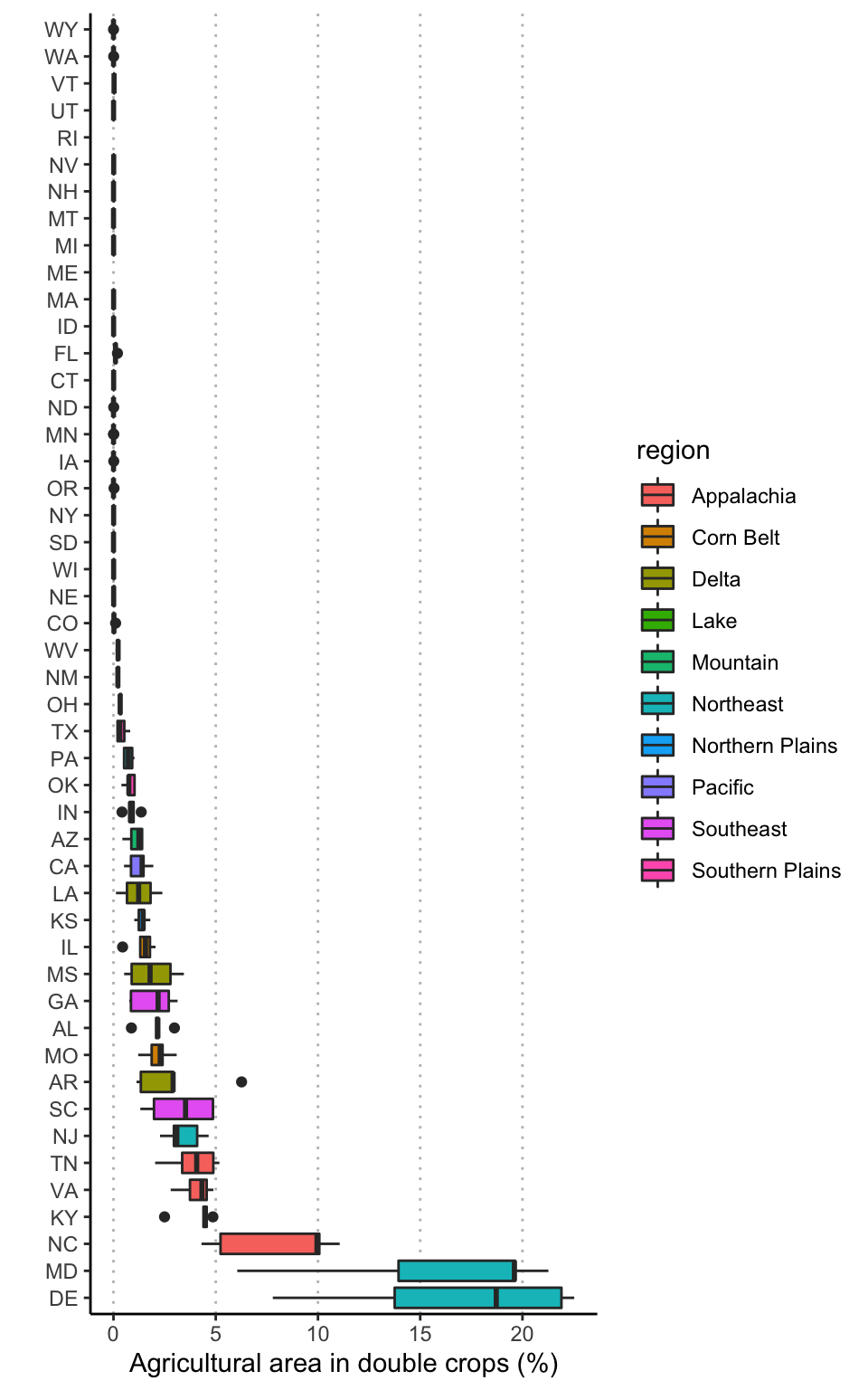
Describe unsurveyed crops
unsurv <- joined_full %>%
  filter(lc_cat == "Not_surveyed") %>%
  group_by(region, state, value, Categories) %>%
  summarise(count = median(count)) %>%
  arrange(state, -count)
## `summarise()` has grouped output by 'region', 'state', 'value'. You can override using the `.groups` argument.unsurv_sum <- unsurv %>%
group_by(Categories) %>%
summarise(count = sum(count))This R Markdown site was created with workflowr