Generate state-by-crop acreage data
Maggie Douglas
Last updated: 2020-07-08
Purpose
This code organizes USDA data on crop acreage into state-crop-year combinations to correspond to those used in USGS pesticide data.
Note As of now this code only extracts data for 1997-2017, because Census data from 1992 are not available through QuickStats.
Data sources
Data sources are described in the data extraction code and the crop key code.
Libraries & functions
library(tidyverse)
library(data.table)
library(latticeExtra)
library(grid)

# function to fix USDA acreage data stored as character
acreNum<-function(x){
  as.numeric(as.character(gsub(",", "", x)))
}
Load data
crop_data <- read.csv("../output_big/nass_survey/qs.crops.ac.st_20200404.csv")
crop_data$acresNum <- acreNum(crop_data$VALUE) # remove commas in acreage data
Warning in acreNum(crop_data$VALUE): NAs introduced by coercioncrop_data$SHORT_DESC <- as.character(crop_data$SHORT_DESC)
str(crop_data)'data.frame': 315934 obs. of 41 variables:
$ X : int 1 2 3 4 5 6 7 8 9 10 ...
$ SOURCE_DESC : Factor w/ 2 levels "CENSUS","SURVEY": 2 2 2 2 2 2 2 1 1 1 ...
$ SECTOR_DESC : Factor w/ 1 level "CROPS": 1 1 1 1 1 1 1 1 1 1 ...
$ GROUP_DESC : Factor w/ 5 levels "CROP TOTALS",..: 2 2 2 2 2 2 2 2 2 2 ...
$ COMMODITY_DESC : Factor w/ 182 levels "ALMONDS","AMARANTH",..: 11 11 11 11 11 11 11 11 11 11 ...
$ CLASS_DESC : Factor w/ 254 levels "(EXCL ALFALFA & WILD)",..: 19 19 19 19 19 19 19 19 19 19 ...
$ PRODN_PRACTICE_DESC : Factor w/ 20 levels "ALL PRODUCTION PRACTICES",..: 1 1 1 1 1 1 1 1 1 1 ...
$ UTIL_PRACTICE_DESC : Factor w/ 18 levels "ALL UTILIZATION PRACTICES",..: 1 1 1 1 1 1 1 1 1 1 ...
$ STATISTICCAT_DESC : Factor w/ 11 levels "AREA","AREA BEARING",..: 5 5 5 5 5 5 5 5 5 5 ...
$ UNIT_DESC : Factor w/ 1 level "ACRES": 1 1 1 1 1 1 1 1 1 1 ...
$ SHORT_DESC : chr "BARLEY - ACRES HARVESTED" "BARLEY - ACRES HARVESTED" "BARLEY - ACRES HARVESTED" "BARLEY - ACRES HARVESTED" ...
$ DOMAIN_DESC : Factor w/ 1 level "TOTAL": 1 1 1 1 1 1 1 1 1 1 ...
$ DOMAINCAT_DESC : Factor w/ 1 level "NOT SPECIFIED": 1 1 1 1 1 1 1 1 1 1 ...
$ AGG_LEVEL_DESC : Factor w/ 1 level "STATE": 1 1 1 1 1 1 1 1 1 1 ...
$ STATE_ANSI : int 1 1 1 1 1 1 1 1 1 1 ...
$ STATE_FIPS_CODE : int 1 1 1 1 1 1 1 1 1 1 ...
$ STATE_ALPHA : Factor w/ 51 levels "AK","AL","AR",..: 2 2 2 2 2 2 2 2 2 2 ...
$ STATE_NAME : Factor w/ 51 levels "ALABAMA","ALASKA",..: 1 1 1 1 1 1 1 1 1 1 ...
$ ASD_CODE : logi NA NA NA NA NA NA ...
$ ASD_DESC : logi NA NA NA NA NA NA ...
$ COUNTY_ANSI : logi NA NA NA NA NA NA ...
$ COUNTY_CODE : logi NA NA NA NA NA NA ...
$ COUNTY_NAME : logi NA NA NA NA NA NA ...
$ REGION_DESC : logi NA NA NA NA NA NA ...
$ ZIP_5 : logi NA NA NA NA NA NA ...
$ WATERSHED_CODE : int 0 0 0 0 0 0 0 0 0 0 ...
$ WATERSHED_DESC : logi NA NA NA NA NA NA ...
$ CONGR_DISTRICT_CODE : logi NA NA NA NA NA NA ...
$ COUNTRY_CODE : int 9000 9000 9000 9000 9000 9000 9000 9000 9000 9000 ...
$ COUNTRY_NAME : Factor w/ 1 level "UNITED STATES": 1 1 1 1 1 1 1 1 1 1 ...
$ LOCATION_DESC : Factor w/ 51 levels "ALABAMA","ALASKA",..: 1 1 1 1 1 1 1 1 1 1 ...
$ YEAR : int 1943 1944 1945 1946 1947 1948 1949 2002 1997 2012 ...
$ FREQ_DESC : Factor w/ 2 levels "ANNUAL","SEASON": 1 1 1 1 1 1 1 1 1 1 ...
$ BEGIN_CODE : int 0 0 0 0 0 0 0 0 0 0 ...
$ END_CODE : int 0 0 0 0 0 0 0 0 0 0 ...
$ REFERENCE_PERIOD_DESC: Factor w/ 23 levels "FALL - SEP FORECAST",..: 5 5 5 5 5 5 5 5 5 5 ...
$ WEEK_ENDING : logi NA NA NA NA NA NA ...
$ LOAD_TIME : Factor w/ 276 levels "1990-06-15 12:06:17",..: 19 19 19 19 19 19 19 19 19 40 ...
$ VALUE : Factor w/ 33373 levels "(1)","(D)","(NA)",..: 23476 23476 9577 9577 9 9577 9577 27981 15514 27836 ...
$ CV_. : Factor w/ 1001 levels "","(D)","(H)",..: 1 1 1 1 1 1 1 1 1 981 ...
$ acresNum : num 5000 5000 2000 2000 1000 2000 2000 665 29 653 ...econ_data <- read.csv("../output_big/nass_survey/qs.economics.ac.st_20200404.csv")
econ_data$acresNum <- acreNum(econ_data$VALUE) # remove commas in acreage dataWarning in acreNum(econ_data$VALUE): NAs introduced by coercionecon_data$SHORT_DESC <- as.character(econ_data$SHORT_DESC)
str(econ_data)'data.frame': 6432 obs. of 41 variables:
$ X : int 1 2 3 4 5 6 7 8 9 10 ...
$ SOURCE_DESC : Factor w/ 1 level "CENSUS": 1 1 1 1 1 1 1 1 1 1 ...
$ SECTOR_DESC : Factor w/ 1 level "ECONOMICS": 1 1 1 1 1 1 1 1 1 1 ...
$ GROUP_DESC : Factor w/ 1 level "FARMS & LAND & ASSETS": 1 1 1 1 1 1 1 1 1 1 ...
$ COMMODITY_DESC : Factor w/ 2 levels "AG LAND","LAND AREA": 1 1 1 1 1 1 1 1 1 1 ...
$ CLASS_DESC : Factor w/ 17 levels "(EXCL CROPLAND & PASTURELAND & WOODLAND)",..: 10 10 10 10 10 10 10 10 10 10 ...
$ PRODN_PRACTICE_DESC : Factor w/ 26 levels "ALL PRODUCTION PRACTICES",..: 4 4 4 4 4 4 4 4 4 4 ...
$ UTIL_PRACTICE_DESC : Factor w/ 1 level "ALL UTILIZATION PRACTICES": 1 1 1 1 1 1 1 1 1 1 ...
$ STATISTICCAT_DESC : Factor w/ 1 level "AREA": 1 1 1 1 1 1 1 1 1 1 ...
$ UNIT_DESC : Factor w/ 1 level "ACRES": 1 1 1 1 1 1 1 1 1 1 ...
$ SHORT_DESC : chr "AG LAND, CROPLAND, PASTURED ONLY, IRRIGATED - ACRES" "AG LAND, CROPLAND, PASTURED ONLY, IRRIGATED - ACRES" "AG LAND, CROPLAND, PASTURED ONLY, IRRIGATED - ACRES" "AG LAND, CROPLAND, PASTURED ONLY, IRRIGATED - ACRES" ...
$ DOMAIN_DESC : Factor w/ 1 level "TOTAL": 1 1 1 1 1 1 1 1 1 1 ...
$ DOMAINCAT_DESC : Factor w/ 1 level "NOT SPECIFIED": 1 1 1 1 1 1 1 1 1 1 ...
$ AGG_LEVEL_DESC : Factor w/ 1 level "STATE": 1 1 1 1 1 1 1 1 1 1 ...
$ STATE_ANSI : int 1 4 4 5 6 6 8 8 9 12 ...
$ STATE_FIPS_CODE : int 1 4 4 5 6 6 8 8 9 12 ...
$ STATE_ALPHA : Factor w/ 50 levels "AK","AL","AR",..: 2 4 4 3 5 5 6 6 7 9 ...
$ STATE_NAME : Factor w/ 50 levels "ALABAMA","ALASKA",..: 1 3 3 4 5 5 6 6 7 9 ...
$ ASD_CODE : logi NA NA NA NA NA NA ...
$ ASD_DESC : logi NA NA NA NA NA NA ...
$ COUNTY_ANSI : logi NA NA NA NA NA NA ...
$ COUNTY_CODE : logi NA NA NA NA NA NA ...
$ COUNTY_NAME : logi NA NA NA NA NA NA ...
$ REGION_DESC : logi NA NA NA NA NA NA ...
$ ZIP_5 : logi NA NA NA NA NA NA ...
$ WATERSHED_CODE : int 0 0 0 0 0 0 0 0 0 0 ...
$ WATERSHED_DESC : logi NA NA NA NA NA NA ...
$ CONGR_DISTRICT_CODE : logi NA NA NA NA NA NA ...
$ COUNTRY_CODE : int 9000 9000 9000 9000 9000 9000 9000 9000 9000 9000 ...
$ COUNTRY_NAME : Factor w/ 1 level "UNITED STATES": 1 1 1 1 1 1 1 1 1 1 ...
$ LOCATION_DESC : Factor w/ 50 levels "ALABAMA","ALASKA",..: 1 3 3 4 5 5 6 6 7 9 ...
$ YEAR : int 2018 2013 2018 2018 2013 2018 2013 2018 2013 2013 ...
$ FREQ_DESC : Factor w/ 1 level "ANNUAL": 1 1 1 1 1 1 1 1 1 1 ...
$ BEGIN_CODE : int 0 0 0 0 0 0 0 0 0 0 ...
$ END_CODE : int 0 0 0 0 0 0 0 0 0 0 ...
$ REFERENCE_PERIOD_DESC: Factor w/ 1 level "YEAR": 1 1 1 1 1 1 1 1 1 1 ...
$ WEEK_ENDING : logi NA NA NA NA NA NA ...
$ LOAD_TIME : Factor w/ 4 levels "2012-01-01 00:00:00",..: 4 2 4 4 2 4 2 4 2 2 ...
$ VALUE : Factor w/ 6255 levels "(D)","1,001,543",..: 1156 4903 3839 4357 1143 2390 2347 5057 1300 1417 ...
$ CV_. : Factor w/ 518 levels "","(D)","(H)",..: 194 1 403 33 1 440 1 263 1 1 ...
$ acresNum : num 120 6001 4661 5 12795 ...crop_key <- read.csv("../keys/crop_key_summary.csv")
crop_key$SHORT_DESC <- as.character(crop_key$SHORT_DESC)Subset data
Select crop acreage that meets the following conditions:
- Annual estimate
- 1992 or later
- Exclude California, Hawaii, Alaska, and “other states”
- California data treated separately, see Baker & Stone (2015)
- Pesticide data only for the contiguous US
- Remove acreage data for crops/categories not represented in USGS data
- Check that each combination of
STATE,YEAR, andSHORT_DESCis represented only once in the dataset (guards against mistakes in data processing)
crop_data_sum <- crop_data %>%
  rbind(econ_data) %>%
  filter(FREQ_DESC=="ANNUAL"&
          REFERENCE_PERIOD_DESC=="YEAR" &
          (YEAR>1991) &
           (STATE_ALPHA!="CA" & STATE_ALPHA!="HI" &
              STATE_ALPHA!="AK" & STATE_ALPHA!="OT")) %>%
  left_join(crop_key, by="SHORT_DESC") %>%
  group_by(SOURCE_DESC, STATE_ANSI, STATE_ALPHA, STATE_NAME, YEAR, SHORT_DESC, e_pest_name, USGS_group) %>%
  summarise(acres = sum(acresNum, na.rm=TRUE),
            acres_n = length(which(!is.na(acresNum))),
            acres_NA = length(which(is.na(acresNum)))) %>%
  filter(!is.na(USGS_group)) %>%
  gather(temp, score, starts_with("acres")) %>%
  unite(temp1, SOURCE_DESC, temp, sep = "_") %>%
  spread(temp1, score) %>%
  mutate(cen_surv_diff_perc = ((SURVEY_acres-CENSUS_acres)/CENSUS_acres)*100,
         cen_surv_perc = (SURVEY_acres/CENSUS_acres)*100,
         cen_surv_diff = SURVEY_acres - CENSUS_acres)

summary(crop_data_sum$CENSUS_acres_n) # no rows with > 1 contributing data point
Min. 1st Qu. Median Mean 3rd Qu. Max. NA's
0.000 1.000 1.000 0.882 1.000 1.000 9872 summary(crop_data_sum$SURVEY_acres_n) Min. 1st Qu. Median Mean 3rd Qu. Max. NA's
0.000 1.000 1.000 0.994 1.000 1.000 11221 Check Census vs. Survey
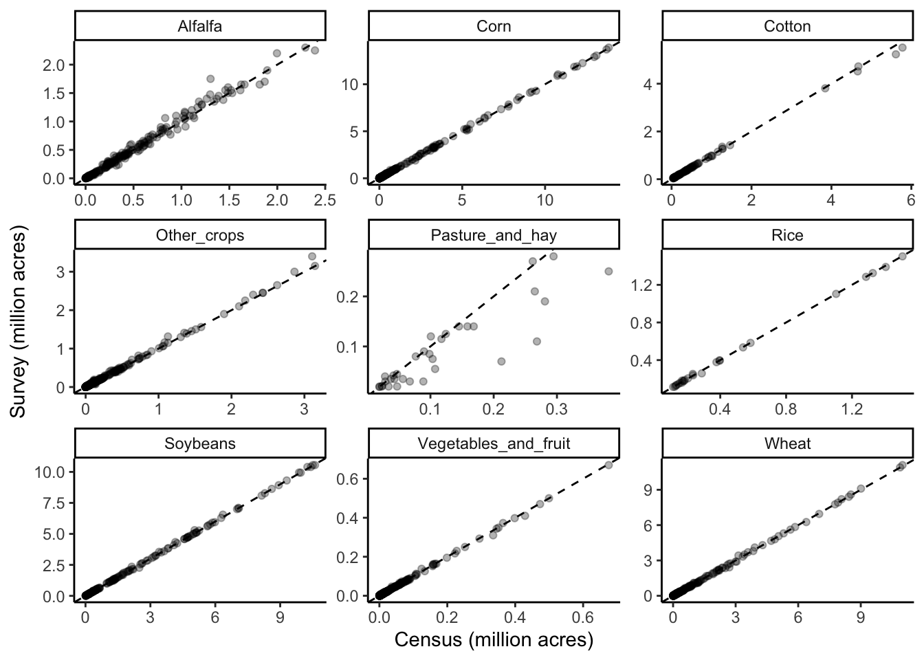
Notes
- These graphs compare estimates from the Census and Survey for those years when estimates are availabe from both data sources.
- Each dot represents a combination of data item (
SHORT_DESC), state, and year - They are grouped by USGS crop category
- In absolute terms, the two data sources are very similar, with the exception of Pasture & Hay where the Survey estimate tends to be lower than the Census estimate (this likely has to do with categories that do not align well between the two datasets).
Generate acreage dataset
Select crop acreage that meets the following conditions:
- Annual estimate
- 1992 or later
- Exclude California, Hawaii, Alaska, and “other states”
- California data treated separately, see Baker & Stone (2015)
- Remove acreage data for crops/categories not represented in USGS data
- Add ‘economic’ dataset to ‘crop’ dataset
Then, generate an acreage dataset for combinations of crop, state, and year, using the following rules:
- Census data is used in Census years (1997,2002,2007,2012,2017)
- Survey data is used to fill in intervening years, when available
- Missing data between the two estimates is estimated using interpolation
- Missing data at the end of the time series is estimated from the most recent available year
Subset appropriate data
cen_yrs <- c(1997,2002,2007,2012,2017) # store census years
non_cen_yrs <- c(1992:1996,1998:2001,2003:2006,2008:2011,2013:2016) # store non-census years

crop_data_full <- crop_data %>%
  rbind(econ_data) %>%
  filter(FREQ_DESC=="ANNUAL"&
          REFERENCE_PERIOD_DESC=="YEAR" &
          (YEAR>1991) &
           (STATE_ALPHA!="CA" & STATE_ALPHA!="HI" &
              STATE_ALPHA!="AK" & STATE_ALPHA!="OT") &
           ((SOURCE_DESC=="CENSUS" & YEAR %in% cen_yrs)|
            SOURCE_DESC=="SURVEY" & YEAR %in% non_cen_yrs)) %>%
  full_join(crop_key, by="SHORT_DESC") %>%
  group_by(SOURCE_DESC,STATE_ANSI,STATE_ALPHA,STATE_NAME,YEAR, SHORT_DESC, e_pest_name, USGS_group) %>%
  summarise(acres = sum(acresNum, na.rm=TRUE),
            acres_n = length(which(!is.na(acresNum))),
            acres_NA = length(which(is.na(acresNum)))) %>%
  filter(!is.na(USGS_group) & acres_n != 0) # filter out 'false' zeroes & crops not in a USGS group

# check that distribution across sources & years is correct
with(crop_data_full, table(SOURCE_DESC,YEAR))
Interpolate to fill gaps
Example
# Example interpolation

state <- "NJ"
crop <- "ASPARAGUS - ACRES HARVESTED"

test<-subset(crop_data_full, SHORT_DESC==crop &
                   STATE_ALPHA==state)
test$pch <- NA
test$pch[test$SOURCE_DESC=="CENSUS"] <- 1
test$pch[test$SOURCE_DESC=="SURVEY"] <- 12
with(test, plot(acres~YEAR, xlim=c(1992,2017), pch=pch))
points(approx(test$YEAR, test$acres, method="linear", rule=2, xout=seq(1992,2017,by=1)), col=4,pch="*")
Full dataset
This code takes several minutes to run
# Split data into separate dataframes by state & SHORT_DESC name (i.e. data item)
crop_state <- as.factor(paste(crop_data_full$SHORT_DESC,crop_data_full$STATE_ALPHA))
crop_split_state <- split(as.data.frame(crop_data_full), f=crop_state)

# This code interpolates values for missing year-state-crop combinations from 1997-2017, for those combinations that have at least two years of data, and returns a new dataframe with the original and interpolated values combined
y <- NULL
for(i in 1:length(crop_split_state))
{
  if (length(crop_split_state[[i]]$acres) > 1) {
    df1 = crop_split_state[[i]]
    temp <- as.data.frame(approx(df1$YEAR, df1$acres, method="linear", xout=seq(1997,2017,by=1), rule=2))
  temp$SHORT_DESC <- as.character(levels(factor(df1$SHORT_DESC)))
  temp$STATE_ALPHA <- as.character(levels(factor(df1$STATE_ALPHA)))
  temp$STATE_ANSI <- as.character(levels(factor(df1$STATE_ANSI)))
  temp$interp <- "yes"
  y <- rbind(y,temp)
  }
  else {
   df2 = crop_split_state[[i]]
   temp <- select(df2, YEAR, acres, SHORT_DESC, STATE_ALPHA, STATE_ANSI)
   colnames(temp)[1] <- "x"
   colnames(temp)[2] <- "y"
   temp$interp <- "no"
   y <- rbind(y,temp)
}
}

colnames(y)[1] <- "YEAR" # fix column names
colnames(y)[2] <- "acres"

# Create a key to add sources back in
source_key <- select(as.data.frame(crop_data_full), STATE_ALPHA, YEAR, SHORT_DESC, SOURCE_DESC)

# Join acreage data with source information
y$STATE_ALPHA <- as.character(y$STATE_ALPHA)
source_key$STATE_ALPHA <- as.character(source_key$STATE_ALPHA)
crop_data_interp <- left_join(y, source_key, by=c("STATE_ALPHA", "YEAR", "SHORT_DESC")) %>%
  mutate(ha = acres*0.404686) %>%
  select(-acres)

# Replace NA source values with 'interp' to indicate interpolated
levels(crop_data_interp$SOURCE_DESC) <- c("CENSUS","SURVEY","interp")
crop_data_interp$SOURCE_DESC[is.na(crop_data_interp$SOURCE_DESC)] <- "interp"

str(crop_data_interp) # check results
Graph area data by USDA crop
This code takes several minutes to run
# Make and store graphs showing full dataset by state, year, and crop
crop_state <- split(as.data.frame(crop_data_interp), f=crop_data_interp$SHORT_DESC)

colors <- c(CENSUS = "black", SURVEY = "blue", interp = "lightblue")

pdf("../output/crops-by-state-yr-updated.pdf",
    width=12, height=8)
for(i in 1:length(crop_state))
{
  df1 = as.data.frame(crop_state[[i]])
  plot <- ggplot(df1, aes(x=YEAR, y=ha, colour=SOURCE_DESC)) +
            geom_point() +
            ylab("Hectares") + xlab("") +
            facet_wrap(~STATE_ALPHA) +
            scale_colour_manual(values = colors) +
            ggtitle(levels(factor(df1$SHORT_DESC))) +
            theme_classic()
  print(plot)
}
dev.off()
Add USGS categories
crop_data_interp <- left_join(crop_data_interp, crop_key, by="SHORT_DESC")Graph acreage by USGS group
# Make and store graphs showing full dataset by state, year, and crop
group_state <- crop_data_interp %>%
  group_by(YEAR, STATE_ALPHA, STATE_ANSI, USGS_group) %>%
  summarise(ha_sum = sum(ha))

group_state_split <- split(as.data.frame(group_state), f=group_state$USGS_group)

pdf("../output/groups-by-state-yr-updated.pdf",
    width=12, height=8)
for(i in 1:length(group_state_split))
{
  df1 = as.data.frame(group_state_split[[i]])
  plot <- ggplot(df1, aes(x=YEAR, y=ha_sum)) +
            geom_point() +
            ylab("Hectares") + xlab("") +
           facet_wrap(~STATE_ALPHA) +
            ggtitle(levels(factor(df1$USGS_group))) +
            theme_classic()
  print(plot)
}
dev.off()
Export data
write.csv(crop_data_interp, "../output_big/hectares_state_usda_usgs_20200404.csv",
          row.names=FALSE)
Session information
sessionInfo()R version 3.6.1 (2019-07-05)
Platform: x86_64-apple-darwin15.6.0 (64-bit)
Running under: macOS High Sierra 10.13.6
Matrix products: default
BLAS: /Library/Frameworks/R.framework/Versions/3.6/Resources/lib/libRblas.0.dylib
LAPACK: /Library/Frameworks/R.framework/Versions/3.6/Resources/lib/libRlapack.dylib
locale:
[1] en_US.UTF-8/en_US.UTF-8/en_US.UTF-8/C/en_US.UTF-8/en_US.UTF-8
attached base packages:
[1] grid stats graphics grDevices utils datasets methods
[8] base
other attached packages:
[1] latticeExtra_0.6-28 RColorBrewer_1.1-2 lattice_0.20-38
[4] data.table_1.12.2 forcats_0.4.0 stringr_1.4.0
[7] dplyr_0.8.3 purrr_0.3.2 readr_1.3.1
[10] tidyr_0.8.3 tibble_2.1.3 ggplot2_3.2.0
[13] tidyverse_1.2.1
loaded via a namespace (and not attached):
[1] Rcpp_1.0.1 cellranger_1.1.0 pillar_1.4.2 compiler_3.6.1
[5] tools_3.6.1 zeallot_0.1.0 digest_0.6.20 lubridate_1.7.4
[9] jsonlite_1.6 evaluate_0.14 nlme_3.1-140 gtable_0.3.0
[13] pkgconfig_2.0.2 rlang_0.4.0 cli_1.1.0 rstudioapi_0.10
[17] yaml_2.2.0 haven_2.1.1 xfun_0.8 withr_2.1.2
[21] xml2_1.2.0 httr_1.4.0 knitr_1.23 vctrs_0.2.0
[25] generics_0.0.2 hms_0.5.0 tidyselect_0.2.5 glue_1.3.1
[29] R6_2.4.0 readxl_1.3.1 rmarkdown_1.14 modelr_0.1.4
[33] magrittr_1.5 backports_1.1.4 scales_1.0.0 htmltools_0.3.6
[37] rvest_0.3.4 assertthat_0.2.1 colorspace_1.4-1 labeling_0.3
[41] stringi_1.4.3 lazyeval_0.2.2 munsell_0.5.0 broom_0.5.2
[45] crayon_1.3.4 This R Markdown site was created with workflowr