Generate California crop acreage data
Maggie Douglas
Last updated: 2020-07-08
Purpose
This code organizes USDA data on California crop acreage into crop-year combinations to correspond to those used in USGS pesticide data.
Note: As of now this code only extracts data for 1997-2017, because Census data from 1992 are not available through QuickStats.
Data sources
Data sources are described in the data extraction code and the crop key code.
Libraries & functions
library(tidyverse)
library(data.table)
library(latticeExtra)
library(grid)

# function to fix USDA acreage data stored as character
acreNum<-function(x){
  as.numeric(as.character(gsub(",", "", x)))
}
Load data
crop_data <- read.csv("../output_big/nass_survey/qs.crops.ac.st_20200404.csv")
crop_data$acresNum <- acreNum(crop_data$VALUE) # remove commas in acreage data
Warning in acreNum(crop_data$VALUE): NAs introduced by coercioncrop_data$SHORT_DESC <- as.character(crop_data$SHORT_DESC)
str(crop_data)'data.frame': 315934 obs. of 41 variables:
$ X : int 1 2 3 4 5 6 7 8 9 10 ...
$ SOURCE_DESC : Factor w/ 2 levels "CENSUS","SURVEY": 2 2 2 2 2 2 2 1 1 1 ...
$ SECTOR_DESC : Factor w/ 1 level "CROPS": 1 1 1 1 1 1 1 1 1 1 ...
$ GROUP_DESC : Factor w/ 5 levels "CROP TOTALS",..: 2 2 2 2 2 2 2 2 2 2 ...
$ COMMODITY_DESC : Factor w/ 182 levels "ALMONDS","AMARANTH",..: 11 11 11 11 11 11 11 11 11 11 ...
$ CLASS_DESC : Factor w/ 254 levels "(EXCL ALFALFA & WILD)",..: 19 19 19 19 19 19 19 19 19 19 ...
$ PRODN_PRACTICE_DESC : Factor w/ 20 levels "ALL PRODUCTION PRACTICES",..: 1 1 1 1 1 1 1 1 1 1 ...
$ UTIL_PRACTICE_DESC : Factor w/ 18 levels "ALL UTILIZATION PRACTICES",..: 1 1 1 1 1 1 1 1 1 1 ...
$ STATISTICCAT_DESC : Factor w/ 11 levels "AREA","AREA BEARING",..: 5 5 5 5 5 5 5 5 5 5 ...
$ UNIT_DESC : Factor w/ 1 level "ACRES": 1 1 1 1 1 1 1 1 1 1 ...
$ SHORT_DESC : chr "BARLEY - ACRES HARVESTED" "BARLEY - ACRES HARVESTED" "BARLEY - ACRES HARVESTED" "BARLEY - ACRES HARVESTED" ...
$ DOMAIN_DESC : Factor w/ 1 level "TOTAL": 1 1 1 1 1 1 1 1 1 1 ...
$ DOMAINCAT_DESC : Factor w/ 1 level "NOT SPECIFIED": 1 1 1 1 1 1 1 1 1 1 ...
$ AGG_LEVEL_DESC : Factor w/ 1 level "STATE": 1 1 1 1 1 1 1 1 1 1 ...
$ STATE_ANSI : int 1 1 1 1 1 1 1 1 1 1 ...
$ STATE_FIPS_CODE : int 1 1 1 1 1 1 1 1 1 1 ...
$ STATE_ALPHA : Factor w/ 51 levels "AK","AL","AR",..: 2 2 2 2 2 2 2 2 2 2 ...
$ STATE_NAME : Factor w/ 51 levels "ALABAMA","ALASKA",..: 1 1 1 1 1 1 1 1 1 1 ...
$ ASD_CODE : logi NA NA NA NA NA NA ...
$ ASD_DESC : logi NA NA NA NA NA NA ...
$ COUNTY_ANSI : logi NA NA NA NA NA NA ...
$ COUNTY_CODE : logi NA NA NA NA NA NA ...
$ COUNTY_NAME : logi NA NA NA NA NA NA ...
$ REGION_DESC : logi NA NA NA NA NA NA ...
$ ZIP_5 : logi NA NA NA NA NA NA ...
$ WATERSHED_CODE : int 0 0 0 0 0 0 0 0 0 0 ...
$ WATERSHED_DESC : logi NA NA NA NA NA NA ...
$ CONGR_DISTRICT_CODE : logi NA NA NA NA NA NA ...
$ COUNTRY_CODE : int 9000 9000 9000 9000 9000 9000 9000 9000 9000 9000 ...
$ COUNTRY_NAME : Factor w/ 1 level "UNITED STATES": 1 1 1 1 1 1 1 1 1 1 ...
$ LOCATION_DESC : Factor w/ 51 levels "ALABAMA","ALASKA",..: 1 1 1 1 1 1 1 1 1 1 ...
$ YEAR : int 1943 1944 1945 1946 1947 1948 1949 2002 1997 2012 ...
$ FREQ_DESC : Factor w/ 2 levels "ANNUAL","SEASON": 1 1 1 1 1 1 1 1 1 1 ...
$ BEGIN_CODE : int 0 0 0 0 0 0 0 0 0 0 ...
$ END_CODE : int 0 0 0 0 0 0 0 0 0 0 ...
$ REFERENCE_PERIOD_DESC: Factor w/ 23 levels "FALL - SEP FORECAST",..: 5 5 5 5 5 5 5 5 5 5 ...
$ WEEK_ENDING : logi NA NA NA NA NA NA ...
$ LOAD_TIME : Factor w/ 276 levels "1990-06-15 12:06:17",..: 19 19 19 19 19 19 19 19 19 40 ...
$ VALUE : Factor w/ 33373 levels "(1)","(D)","(NA)",..: 23476 23476 9577 9577 9 9577 9577 27981 15514 27836 ...
$ CV_. : Factor w/ 1001 levels "","(D)","(H)",..: 1 1 1 1 1 1 1 1 1 981 ...
$ acresNum : num 5000 5000 2000 2000 1000 2000 2000 665 29 653 ...econ_data <- read.csv("../output_big/nass_survey/qs.economics.ac.st_20200404.csv")
econ_data$acresNum <- acreNum(econ_data$VALUE) # remove commas in acreage dataWarning in acreNum(econ_data$VALUE): NAs introduced by coercionecon_data$SHORT_DESC <- as.character(econ_data$SHORT_DESC)
str(econ_data)'data.frame': 6432 obs. of 41 variables:
$ X : int 1 2 3 4 5 6 7 8 9 10 ...
$ SOURCE_DESC : Factor w/ 1 level "CENSUS": 1 1 1 1 1 1 1 1 1 1 ...
$ SECTOR_DESC : Factor w/ 1 level "ECONOMICS": 1 1 1 1 1 1 1 1 1 1 ...
$ GROUP_DESC : Factor w/ 1 level "FARMS & LAND & ASSETS": 1 1 1 1 1 1 1 1 1 1 ...
$ COMMODITY_DESC : Factor w/ 2 levels "AG LAND","LAND AREA": 1 1 1 1 1 1 1 1 1 1 ...
$ CLASS_DESC : Factor w/ 17 levels "(EXCL CROPLAND & PASTURELAND & WOODLAND)",..: 10 10 10 10 10 10 10 10 10 10 ...
$ PRODN_PRACTICE_DESC : Factor w/ 26 levels "ALL PRODUCTION PRACTICES",..: 4 4 4 4 4 4 4 4 4 4 ...
$ UTIL_PRACTICE_DESC : Factor w/ 1 level "ALL UTILIZATION PRACTICES": 1 1 1 1 1 1 1 1 1 1 ...
$ STATISTICCAT_DESC : Factor w/ 1 level "AREA": 1 1 1 1 1 1 1 1 1 1 ...
$ UNIT_DESC : Factor w/ 1 level "ACRES": 1 1 1 1 1 1 1 1 1 1 ...
$ SHORT_DESC : chr "AG LAND, CROPLAND, PASTURED ONLY, IRRIGATED - ACRES" "AG LAND, CROPLAND, PASTURED ONLY, IRRIGATED - ACRES" "AG LAND, CROPLAND, PASTURED ONLY, IRRIGATED - ACRES" "AG LAND, CROPLAND, PASTURED ONLY, IRRIGATED - ACRES" ...
$ DOMAIN_DESC : Factor w/ 1 level "TOTAL": 1 1 1 1 1 1 1 1 1 1 ...
$ DOMAINCAT_DESC : Factor w/ 1 level "NOT SPECIFIED": 1 1 1 1 1 1 1 1 1 1 ...
$ AGG_LEVEL_DESC : Factor w/ 1 level "STATE": 1 1 1 1 1 1 1 1 1 1 ...
$ STATE_ANSI : int 1 4 4 5 6 6 8 8 9 12 ...
$ STATE_FIPS_CODE : int 1 4 4 5 6 6 8 8 9 12 ...
$ STATE_ALPHA : Factor w/ 50 levels "AK","AL","AR",..: 2 4 4 3 5 5 6 6 7 9 ...
$ STATE_NAME : Factor w/ 50 levels "ALABAMA","ALASKA",..: 1 3 3 4 5 5 6 6 7 9 ...
$ ASD_CODE : logi NA NA NA NA NA NA ...
$ ASD_DESC : logi NA NA NA NA NA NA ...
$ COUNTY_ANSI : logi NA NA NA NA NA NA ...
$ COUNTY_CODE : logi NA NA NA NA NA NA ...
$ COUNTY_NAME : logi NA NA NA NA NA NA ...
$ REGION_DESC : logi NA NA NA NA NA NA ...
$ ZIP_5 : logi NA NA NA NA NA NA ...
$ WATERSHED_CODE : int 0 0 0 0 0 0 0 0 0 0 ...
$ WATERSHED_DESC : logi NA NA NA NA NA NA ...
$ CONGR_DISTRICT_CODE : logi NA NA NA NA NA NA ...
$ COUNTRY_CODE : int 9000 9000 9000 9000 9000 9000 9000 9000 9000 9000 ...
$ COUNTRY_NAME : Factor w/ 1 level "UNITED STATES": 1 1 1 1 1 1 1 1 1 1 ...
$ LOCATION_DESC : Factor w/ 50 levels "ALABAMA","ALASKA",..: 1 3 3 4 5 5 6 6 7 9 ...
$ YEAR : int 2018 2013 2018 2018 2013 2018 2013 2018 2013 2013 ...
$ FREQ_DESC : Factor w/ 1 level "ANNUAL": 1 1 1 1 1 1 1 1 1 1 ...
$ BEGIN_CODE : int 0 0 0 0 0 0 0 0 0 0 ...
$ END_CODE : int 0 0 0 0 0 0 0 0 0 0 ...
$ REFERENCE_PERIOD_DESC: Factor w/ 1 level "YEAR": 1 1 1 1 1 1 1 1 1 1 ...
$ WEEK_ENDING : logi NA NA NA NA NA NA ...
$ LOAD_TIME : Factor w/ 4 levels "2012-01-01 00:00:00",..: 4 2 4 4 2 4 2 4 2 2 ...
$ VALUE : Factor w/ 6255 levels "(D)","1,001,543",..: 1156 4903 3839 4357 1143 2390 2347 5057 1300 1417 ...
$ CV_. : Factor w/ 518 levels "","(D)","(H)",..: 194 1 403 33 1 440 1 263 1 1 ...
$ acresNum : num 120 6001 4661 5 12795 ...crop_key_CA <- read.csv("../keys/crop_key_summary_CA.csv")
crop_key_CA$SHORT_DESC <- as.character(crop_key_CA$SHORT_DESC)Subset data
Select crop acreage that meets the following conditions:
- Annual estimate
- 1992 or later
- Only California
- Remove acreage data for crops/categories not represented in USGS data
- Check that each combination of
STATE,YEAR, andSHORT_DESCis represented only once in the dataset (guards against mistakes in data processing)
crop_data_sum <- crop_data %>%
  rbind(econ_data) %>%
  filter(FREQ_DESC=="ANNUAL"&
          REFERENCE_PERIOD_DESC=="YEAR" &
          (YEAR>1991) &
           (STATE_ALPHA=="CA")) %>%
  left_join(crop_key_CA, by="SHORT_DESC") %>%
  group_by(SOURCE_DESC, STATE_ANSI, STATE_ALPHA, STATE_NAME, YEAR, SHORT_DESC, e_pest_name, USGS_group) %>%
  summarise(acres = sum(acresNum, na.rm=TRUE),
            acres_n = length(which(!is.na(acresNum))),
            acres_NA = length(which(is.na(acresNum)))) %>%
  filter(!is.na(USGS_group)) %>%
  gather(temp, score, starts_with("acres")) %>%
  unite(temp1, SOURCE_DESC, temp, sep = "_") %>%
  spread(temp1, score) %>%
  mutate(cen_surv_diff_perc = ((SURVEY_acres-CENSUS_acres)/CENSUS_acres)*100,
         cen_surv_perc = (SURVEY_acres/CENSUS_acres)*100,
         cen_surv_diff = SURVEY_acres - CENSUS_acres)

summary(crop_data_sum$CENSUS_acres_n) # no rows with > 1 contributing data point
Min. 1st Qu. Median Mean 3rd Qu. Max. NA's
0.0000 1.0000 1.0000 0.9317 1.0000 1.0000 584 summary(crop_data_sum$SURVEY_acres_n) Min. 1st Qu. Median Mean 3rd Qu. Max. NA's
0.0000 1.0000 1.0000 0.9986 1.0000 1.0000 455 Check Census vs. Survey
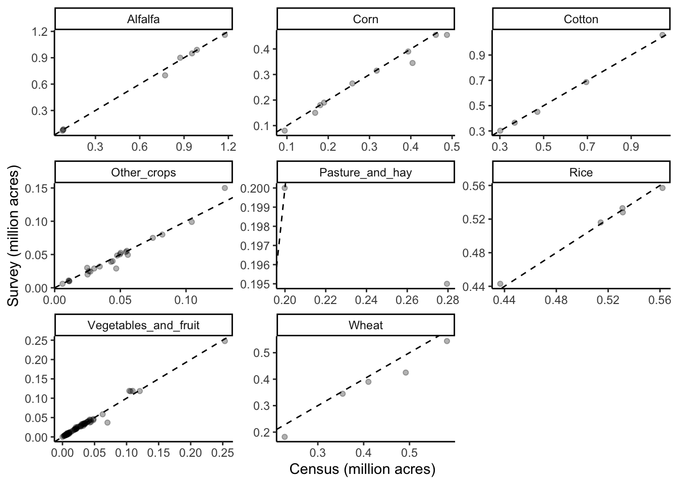
Notes
- These graphs compare estimates from the Census and Survey for those years when estimates are available from both data sources.
- Each dot represents a combination of data item (
SHORT_DESC), state, and year - They are grouped by USGS crop category
- In absolute terms, the two data sources are very similar, with the exception of Pasture & Hay
Generate acreage dataset
Select crop acreage that meets the following conditions:
- Annual estimate
- 1992 or later
- California only
- Remove acreage data for crops/categories not represented in USGS data
- Add ‘economic’ dataset to ‘crop’ dataset
Then, generate an acreage dataset for combinations of crop, state, and year, using the following rules:
- Census data is used in Census years (1997,2002,2007,2012)
- Survey data is used to fill in intervening years, when available
- Missing data between the two estimates is estimated using interpolation
- Missing data at the end of the time series is estimated from the most recent available year
Subset appropriate data
cen_yrs <- c(1997,2002,2007,2012,2017) # store census years
non_cen_yrs <- c(1992:1996,1998:2001,2003:2006,2008:2011,2013:2016) # store non-census years

crop_data_full <- crop_data %>%
  rbind(econ_data) %>%
  filter(FREQ_DESC=="ANNUAL"&
          REFERENCE_PERIOD_DESC=="YEAR" &
          (YEAR>1991) &
           (STATE_ALPHA=="CA") &
           ((SOURCE_DESC=="CENSUS" & YEAR %in% cen_yrs)|
            SOURCE_DESC=="SURVEY" & YEAR %in% non_cen_yrs)) %>%
  full_join(crop_key_CA, by="SHORT_DESC") %>%
  group_by(SOURCE_DESC,STATE_ANSI,STATE_ALPHA,STATE_NAME,YEAR, SHORT_DESC, e_pest_name, USGS_group) %>%
  summarise(acres = sum(acresNum, na.rm=TRUE),
            acres_n = length(which(!is.na(acresNum))),
            acres_NA = length(which(is.na(acresNum)))) %>%
  filter(!is.na(USGS_group) & acres_n != 0) # filter out 'false' zeroes & crops not in a USGS group

# check that distribution across sources & years is correct
with(crop_data_full, table(SOURCE_DESC,YEAR))
Interpolate to fill gaps
Example
# Example interpolation

state <- "CA"
crop <- "ASPARAGUS - ACRES HARVESTED"

test<-subset(crop_data_full, SHORT_DESC==crop &
                   STATE_ALPHA==state)
test$pch <- NA
test$pch[test$SOURCE_DESC=="CENSUS"] <- 1
test$pch[test$SOURCE_DESC=="SURVEY"] <- 12
with(test, plot(acres~YEAR, xlim=c(1992,2017), pch=pch))
points(approx(test$YEAR, test$acres, method="linear", rule=2, xout=seq(1992,2017,by=1)), col=4,pch="*")
Full dataset
This code takes several minutes to run
# Split data into separate dataframes by state & SHORT_DESC name (i.e. data item)
crop_state <- as.factor(paste(crop_data_full$SHORT_DESC,crop_data_full$STATE_ALPHA))
crop_split_state <- split(as.data.frame(crop_data_full), f=crop_state)

# This code interpolates values for missing year-state-crop combinations from 1997-2017, for those combinations that have at least two years of data, and returns a new dataframe with the original and interpolated values combined
y <- NULL
for(i in 1:length(crop_split_state))
{
  if (length(crop_split_state[[i]]$acres) > 1) {
    df1 = crop_split_state[[i]]
    temp <- as.data.frame(approx(df1$YEAR, df1$acres, method="linear", xout=seq(1997,2017,by=1), rule=2))
  temp$SHORT_DESC <- as.character(levels(factor(df1$SHORT_DESC)))
  temp$STATE_ALPHA <- as.character(levels(factor(df1$STATE_ALPHA)))
  temp$STATE_ANSI <- as.character(levels(factor(df1$STATE_ANSI)))
  temp$interp <- "yes"
  y <- rbind(y,temp)
  }
  else {
   df2 = crop_split_state[[i]]
   temp <- select(df2, YEAR, acres, SHORT_DESC, STATE_ALPHA, STATE_ANSI)
   colnames(temp)[1] <- "x"
   colnames(temp)[2] <- "y"
   temp$interp <- "no"
   y <- rbind(y,temp)
}
}

colnames(y)[1] <- "YEAR" # fix column names
colnames(y)[2] <- "acres"

# Create a key to add sources back in
source_key <- select(as.data.frame(crop_data_full), STATE_ALPHA, YEAR, SHORT_DESC, SOURCE_DESC)

# Join acreage data with source information
y$STATE_ALPHA <- as.character(y$STATE_ALPHA)
source_key$STATE_ALPHA <- as.character(source_key$STATE_ALPHA)
crop_data_interp <- left_join(y, source_key, by=c("STATE_ALPHA", "YEAR", "SHORT_DESC")) %>%
  mutate(ha = acres*0.404686) %>%
  select(-acres)

# Replace NA source values with 'interp' to indicate interpolated
levels(crop_data_interp$SOURCE_DESC) <- c("CENSUS","SURVEY","interp")
crop_data_interp$SOURCE_DESC[is.na(crop_data_interp$SOURCE_DESC)] <- "interp"

str(crop_data_interp) # check results
Graph acreage data by USDA crop
This code takes several minutes to run
# Make and store graphs showing full dataset by state, year, and crop
crop_state <- split(as.data.frame(crop_data_interp), f=crop_data_interp$SHORT_DESC)

colors <- c(CENSUS = "black", SURVEY = "blue", interp = "lightblue")

pdf("../output/crops-CA-yr-updated.pdf",
    width=12, height=8)
for(i in 1:length(crop_state))
{
  df1 = as.data.frame(crop_state[[i]])
  plot <- ggplot(df1, aes(x=YEAR, y=ha, colour=SOURCE_DESC)) +
            geom_point() +
            ylab("Hectares") + xlab("") +
            facet_wrap(~STATE_ALPHA) +
            scale_colour_manual(values = colors) +
            ggtitle(levels(factor(df1$SHORT_DESC))) +
            theme_classic()
  print(plot)
}
dev.off()
Add USGS categories
crop_data_interp <- left_join(crop_data_interp, crop_key_CA, by="SHORT_DESC")Graph acreage by USGS group
# Make and store graphs showing full dataset by state, year, and crop
group_state <- crop_data_interp %>%
  group_by(YEAR, STATE_ALPHA, STATE_ANSI, USGS_group) %>%
  summarise(ha_sum = sum(ha))

group_state_split <- split(as.data.frame(group_state), f=group_state$USGS_group)

pdf("../output/groups-CA-yr-updated.pdf",
    width=12, height=8)
for(i in 1:length(group_state_split))
{
  df1 = as.data.frame(group_state_split[[i]])
  plot <- ggplot(df1, aes(x=YEAR, y=ha_sum)) +
            geom_point() +
            ylab("Hectares") + xlab("") +
            ggtitle(levels(factor(df1$USGS_group))) +
            theme_classic()
  print(plot)
}
dev.off()
Export data
write.csv(crop_data_interp, "../output_big/hectares_CA_usda_usgs_20200404.csv",
          row.names=FALSE)
Session information
sessionInfo()R version 3.6.1 (2019-07-05)
Platform: x86_64-apple-darwin15.6.0 (64-bit)
Running under: macOS High Sierra 10.13.6
Matrix products: default
BLAS: /Library/Frameworks/R.framework/Versions/3.6/Resources/lib/libRblas.0.dylib
LAPACK: /Library/Frameworks/R.framework/Versions/3.6/Resources/lib/libRlapack.dylib
locale:
[1] en_US.UTF-8/en_US.UTF-8/en_US.UTF-8/C/en_US.UTF-8/en_US.UTF-8
attached base packages:
[1] grid stats graphics grDevices utils datasets methods
[8] base
other attached packages:
[1] latticeExtra_0.6-28 RColorBrewer_1.1-2 lattice_0.20-38
[4] data.table_1.12.2 forcats_0.4.0 stringr_1.4.0
[7] dplyr_0.8.3 purrr_0.3.2 readr_1.3.1
[10] tidyr_0.8.3 tibble_2.1.3 ggplot2_3.2.0
[13] tidyverse_1.2.1
loaded via a namespace (and not attached):
[1] Rcpp_1.0.1 cellranger_1.1.0 pillar_1.4.2 compiler_3.6.1
[5] tools_3.6.1 zeallot_0.1.0 digest_0.6.20 lubridate_1.7.4
[9] jsonlite_1.6 evaluate_0.14 nlme_3.1-140 gtable_0.3.0
[13] pkgconfig_2.0.2 rlang_0.4.0 cli_1.1.0 rstudioapi_0.10
[17] yaml_2.2.0 haven_2.1.1 xfun_0.8 withr_2.1.2
[21] xml2_1.2.0 httr_1.4.0 knitr_1.23 vctrs_0.2.0
[25] generics_0.0.2 hms_0.5.0 tidyselect_0.2.5 glue_1.3.1
[29] R6_2.4.0 readxl_1.3.1 rmarkdown_1.14 modelr_0.1.4
[33] magrittr_1.5 backports_1.1.4 scales_1.0.0 htmltools_0.3.6
[37] rvest_0.3.4 assertthat_0.2.1 colorspace_1.4-1 labeling_0.3
[41] stringi_1.4.3 lazyeval_0.2.2 munsell_0.5.0 broom_0.5.2
[45] crayon_1.3.4 This R Markdown site was created with workflowr