Calculate Bee Tox Index for state-crop-year combinations
Maggie Douglas
Last updated: 2021-09-29
Purpose
This code uses toxicity data (from EPA, PPDB), pesticide use data (from USGS), and acreage data (from USDA) to derive an estimate of pesticide use in units of honey bee toxicity per acre for combinations of states, years, and crop groups.
Libraries
library(tidyverse)── Attaching packages ──────────────────────────────────────── tidyverse 1.2.1 ──✔ ggplot2 3.2.0 ✔ purrr 0.3.2
✔ tibble 2.1.3 ✔ dplyr 0.8.3
✔ tidyr 1.1.0 ✔ stringr 1.4.0
✔ readr 1.3.1 ✔ forcats 0.4.0── Conflicts ─────────────────────────────────────────── tidyverse_conflicts() ──
✖ dplyr::filter() masks stats::filter()
✖ dplyr::lag() masks stats::lag()Load & organize data
Pesticide data
Data is state-level pesticide use data from the USGS Pesticide National Synthesis Project, available here. There is a ‘low’ estimate and a ‘high’ estimate that differ slightly in the methodology used to estimate missing values. I am using the low estimate to err on the side of being conservative, and because previous studies have found it to be closer to independent estimates.
pest <- read.csv("../data_big/usgs_pesticides/USGS_EpestLOW92to17_CropGroupbyState_06092020.csv")
str(pest)
'data.frame': 185531 obs. of 15 variables:
$ State_FIPS_code : int 1 1 1 1 1 1 1 1 1 1 ...
$ State : Factor w/ 48 levels "Alabama","Arizona",..: 1 1 1 1 1 1 1 1 1 1 ...
$ Compound : Factor w/ 522 levels "1-METHYL CYCLOPROPENE",..: 2 2 2 2 2 2 2 2 2 2 ...
$ Year : int 1992 1993 1994 1995 1996 1997 1998 1999 2000 2001 ...
$ Units : Factor w/ 1 level "kg": 1 1 1 1 1 1 1 1 1 1 ...
$ Corn : num 3775 3951 3324 855 3019 ...
$ Soybeans : num NA NA 66.7 1832.5 21210.5 ...
$ Wheat : num 5129 14390 103 4560 6108 ...
$ Cotton : num NA NA NA NA 3549 ...
$ Vegetables_and_fruit: num 30.3 NA 12.3 4 32.2 ...
$ Rice : num NA NA NA NA NA NA NA NA NA NA ...
$ Orchards_and_grapes : num 134 NA NA 312 217 ...
$ Alfalfa : num NA NA NA NA NA NA NA NA NA NA ...
$ Pasture_and_hay : num 60348 53527 50899 61755 107006 ...
$ Other_crops : num 6838 20476 15174 10223 6213 ...# Reorganize data to long form
pest_long <- pest %>%
gather(Corn,Soybeans,Wheat,Cotton,Vegetables_and_fruit,
Rice,Orchards_and_grapes,Alfalfa,Pasture_and_hay,Other_crops,
key="crop",
value="kg_app",
na.rm=FALSE) %>%
filter(Year > 1996)
# Create new column of compound names to match LD50 data
pest_long$cmpd_usgs <- gsub(",|-| ","",pest_long$Compound)
pest_long$cmpd_usgs <- toupper(pest_long$cmpd_usgs)
# Remove NAs
summary(pest_long) State_FIPS_code State
Min. : 1.00 California: 62840
1st Qu.:17.00 Washington: 42550
Median :30.00 Oregon : 42360
Mean :29.78 Texas : 40780
3rd Qu.:42.00 Georgia : 39380
Max. :56.00 Michigan : 39000
(Other) :1285930
Compound Year Units
2,4-D : 10080 Min. :1997 kg:1552840
ATRAZINE : 10080 1st Qu.:2002
CHLOROTHALONIL : 10080 Median :2007
CHLORPYRIFOS : 10080 Mean :2007
GLYPHOSATE : 10080 3rd Qu.:2012
METOLACHLOR & METOLACHLOR-S: 10080 Max. :2017
(Other) :1492360
crop kg_app cmpd_usgs
Length:1552840 Min. : 0 Length:1552840
Class :character 1st Qu.: 35 Class :character
Mode :character Median : 384 Mode :character
Mean : 29200
3rd Qu.: 3326
Max. :34181135
NA's :1255261 pest_long <- na.omit(pest_long)Crop area data
hectares <- read.csv("../output_big/hectares_state_usda_usgs_20200404.csv")
str(hectares)
'data.frame': 56152 obs. of 9 variables:
$ YEAR : int 1997 1998 1999 2000 2001 2002 2003 2004 2005 2006 ...
$ SHORT_DESC : Factor w/ 86 levels "AG LAND, CROPLAND, (EXCL HARVESTED & PASTURED), CULTIVATED SUMMER FALLOW - ACRES",..: 1 1 1 1 1 1 1 1 1 1 ...
$ STATE_ALPHA: Factor w/ 47 levels "AL","AR","AZ",..: 1 1 1 1 1 1 1 1 1 1 ...
$ STATE_ANSI : int 1 1 1 1 1 1 1 1 1 1 ...
$ interp : Factor w/ 2 levels "no","yes": 2 2 2 2 2 2 2 2 2 2 ...
$ SOURCE_DESC: Factor w/ 3 levels "CENSUS","interp",..: 1 2 2 2 2 1 2 2 2 2 ...
$ ha : num 10256 11078 11900 12722 13544 ...
$ e_pest_name: Factor w/ 58 levels "Alfalfa","Almonds",..: 22 22 22 22 22 22 22 22 22 22 ...
$ USGS_group : Factor w/ 10 levels "Alfalfa","Corn",..: 6 6 6 6 6 6 6 6 6 6 ...hectares_CA <- read.csv("../output_big/hectares_CA_usda_usgs_20200404.csv")
str(hectares_CA)'data.frame': 2444 obs. of 9 variables:
$ YEAR : int 1997 1998 1999 2000 2001 2002 2003 2004 2005 2006 ...
$ SHORT_DESC : Factor w/ 124 levels "AG LAND, CROPLAND, (EXCL HARVESTED & PASTURED), CULTIVATED SUMMER FALLOW - ACRES",..: 1 1 1 1 1 1 1 1 1 1 ...
$ STATE_ALPHA: Factor w/ 1 level "CA": 1 1 1 1 1 1 1 1 1 1 ...
$ STATE_ANSI : int 6 6 6 6 6 6 6 6 6 6 ...
$ interp : Factor w/ 2 levels "no","yes": 2 2 2 2 2 2 2 2 2 2 ...
$ SOURCE_DESC: Factor w/ 3 levels "CENSUS","interp",..: 1 2 2 2 2 1 2 2 2 2 ...
$ ha : num 77381 76778 76175 75572 74969 ...
$ e_pest_name: Factor w/ 100 levels "Alfalfa","Almonds",..: 33 33 33 33 33 33 33 33 33 33 ...
$ USGS_group : Factor w/ 9 levels "Alfalfa","Corn",..: 6 6 6 6 6 6 6 6 6 6 ...# Aggregate area data by USGS crop category
ha_agg <- hectares %>%
group_by(YEAR,STATE_ALPHA,STATE_ANSI,USGS_group) %>%
summarise(ha = sum(ha, na.rm=TRUE))
str(as.data.frame(ha_agg))'data.frame': 8154 obs. of 5 variables:
$ YEAR : int 1996 1997 1997 1997 1997 1997 1997 1997 1997 1997 ...
$ STATE_ALPHA: Factor w/ 47 levels "AL","AR","AZ",..: 29 1 1 1 1 1 1 1 1 1 ...
$ STATE_ANSI : int 35 1 1 1 1 1 1 1 1 1 ...
$ USGS_group : Factor w/ 10 levels "Alfalfa","Corn",..: 5 1 2 3 4 5 6 8 9 10 ...
$ ha : num 364 5297 105266 180111 13151 ...ha_agg_CA <- hectares_CA %>%
group_by(YEAR,STATE_ALPHA,STATE_ANSI,USGS_group) %>%
summarise(ha = sum(ha, na.rm=TRUE))
str(as.data.frame(ha_agg_CA))'data.frame': 189 obs. of 5 variables:
$ YEAR : int 1997 1997 1997 1997 1997 1997 1997 1997 1997 1998 ...
$ STATE_ALPHA: Factor w/ 1 level "CA": 1 1 1 1 1 1 1 1 1 1 ...
$ STATE_ANSI : int 6 6 6 6 6 6 6 6 6 6 ...
$ USGS_group : Factor w/ 9 levels "Alfalfa","Corn",..: 1 2 3 4 5 6 7 8 9 1 ...
$ ha : num 424826 233046 422172 1023300 193151 ...ha_agg_tot <- rbind(ha_agg, ha_agg_CA) %>%
ungroup()
str(as.data.frame(ha_agg_tot))'data.frame': 8343 obs. of 5 variables:
$ YEAR : int 1996 1997 1997 1997 1997 1997 1997 1997 1997 1997 ...
$ STATE_ALPHA: chr "NM" "AL" "AL" "AL" ...
$ STATE_ANSI : int 35 1 1 1 1 1 1 1 1 1 ...
$ USGS_group : chr "Other_crops" "Alfalfa" "Corn" "Cotton" ...
$ ha : num 364 5297 105266 180111 13151 ...LD50 data
ld50 <- read.csv("../output/ld50_usgs_complete_20200609.csv")
str(ld50)
'data.frame': 671 obs. of 13 variables:
$ cmpd_usgs : Factor w/ 523 levels "1METHYLCYCLOPROPENE",..: 1 2 3 4 5 5 6 7 7 8 ...
$ exp_grp : Factor w/ 2 levels "contact","oral": NA NA NA NA 1 2 NA 1 2 1 ...
$ ld50_op : Factor w/ 2 levels "=",">": NA NA NA NA 1 1 NA 1 1 2 ...
$ ld50_n : int NA NA NA NA 2 1 NA 1 1 3 ...
$ cat : Factor w/ 6 levels "F","FUM","H",..: 6 3 3 6 4 4 6 4 4 4 ...
$ cat_grp : Factor w/ 39 levels "I-10A","I-10B",..: NA NA NA NA 31 31 NA 13 13 14 ...
$ class : Factor w/ 28 levels "anthranilic diamide",..: NA NA NA NA 2 2 NA 19 19 28 ...
$ grp_source : Factor w/ 1 level "IRAC": NA NA NA NA 1 1 NA 1 1 1 ...
$ cat_exp_grp: Factor w/ 78 levels "I-10A contact",..: NA NA NA NA 61 62 NA 25 26 27 ...
$ ld50_ugbee : num NA NA NA NA 0.03 ...
$ source : Factor w/ 9 levels "cat_med","ecotox",..: NA NA NA NA 5 2 NA 4 2 5 ...
$ new_2020 : Factor w/ 2 levels "n","y": 1 1 1 1 1 1 2 1 1 1 ...
$ notes : Factor w/ 2 levels "","see Minn Dept Ag - looks high toxicity": 1 1 1 1 1 1 1 1 1 1 ...ld50_ct <- ld50 %>%
filter(exp_grp=="contact") %>% # select contact toxicity
rename("ld50_ugbee_ct" = "ld50_ugbee",
"source_ct" = "source")
ld50_or <- ld50 %>%
filter(exp_grp=="oral") %>% # select oral toxicity
rename("ld50_ugbee_or" = "ld50_ugbee",
"source_or" = "source") %>%
select(cmpd_usgs, ld50_ugbee_or, source_or)
ld50_other <- ld50 %>%
filter(cat %in% c("H","F","PGR","O","FUM"))
ld50_key <- ld50_ct %>%
full_join(ld50_or, by="cmpd_usgs") %>%
bind_rows(ld50_other) %>%
select(cmpd_usgs, ld50_ugbee_ct, ld50_ugbee_or, source_ct, source_or, cat, cat_grp, class, grp_source)
# check relationship between contact and oral LD50 values
with(ld50_key, plot(log(ld50_ugbee_ct)~log(ld50_ugbee_or)))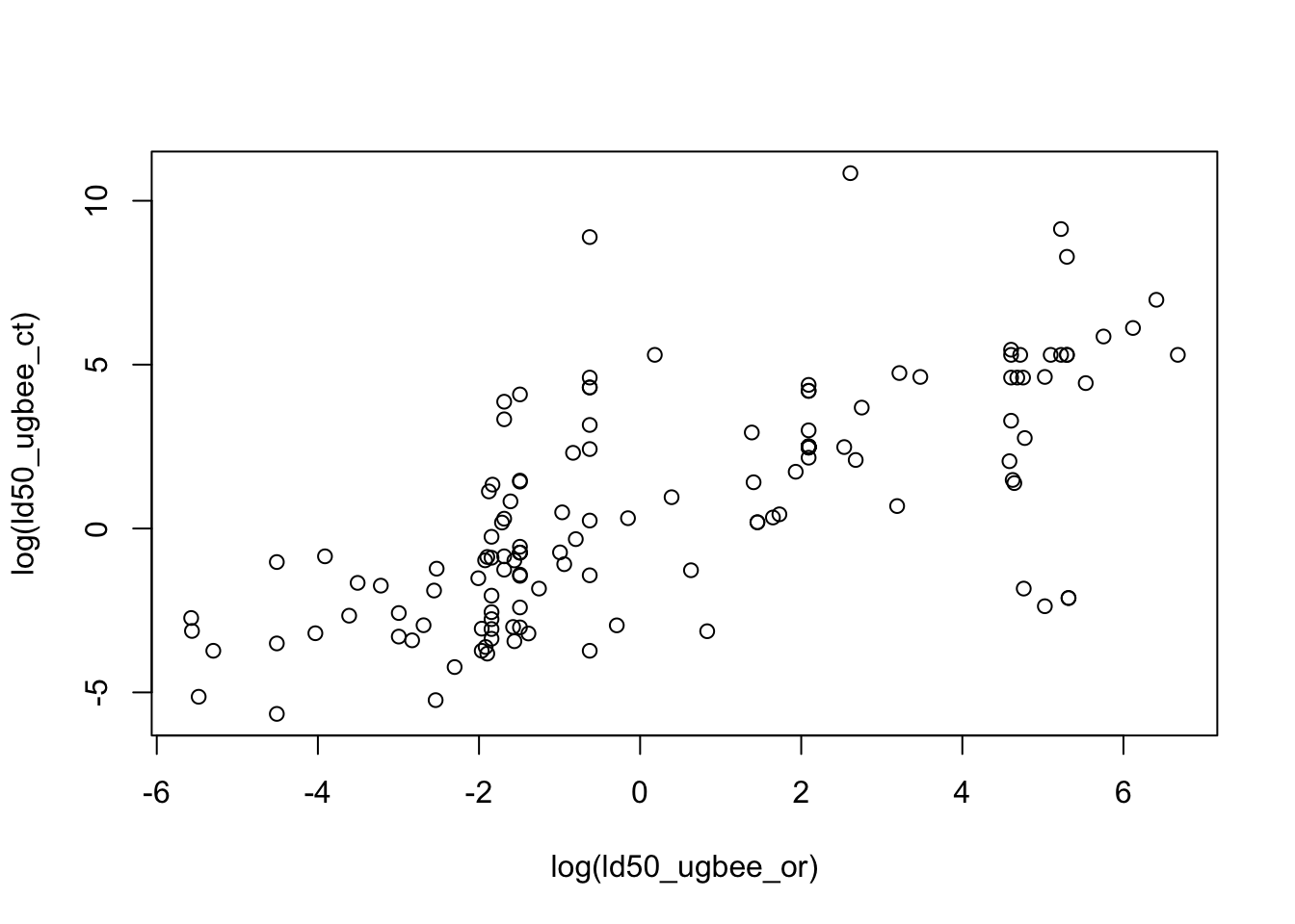
Relate datasets
# Check if all compound names in the pesticide dataset are in the LD50 dataset
check_cmpd <- as.data.frame(unique(pest_long$cmpd_usgs) %in% unique(ld50_key$cmpd_usgs))
check_cmpd$cmpd_usgs <- unique(pest_long$cmpd_usgs)
out <- check_cmpd[check_cmpd==FALSE,]

# Join pesticide data to acreage and LD50 data
data <- pest_long %>%
  full_join(ha_agg_tot, by=c("Year"="YEAR",
                            "State_FIPS_code"="STATE_ANSI",
                            "crop"="USGS_group")) %>%
  left_join(ld50_key, by="cmpd_usgs")

# Examine rows with pesticide data but not area data - appears minor issue (mostly soy in CA)
data_check <- data[is.na(data$ha),]
(sum(data_check$kg_app)/sum(data$kg_app, na.rm=TRUE))*100 # percent kg excluded, nearly zero
[1] 6.086965e-05str(data)'data.frame': 298007 obs. of 18 variables:
$ State_FIPS_code: int 1 1 1 1 1 1 1 1 1 1 ...
$ State : Factor w/ 48 levels "Alabama","Arizona",..: 1 1 1 1 1 1 1 1 1 1 ...
$ Compound : Factor w/ 522 levels "1-METHYL CYCLOPROPENE",..: 2 2 2 2 2 2 2 2 2 2 ...
$ Year : int 1997 1998 1999 2000 2001 2002 2003 2007 2008 2009 ...
$ Units : Factor w/ 1 level "kg": 1 1 1 1 1 1 1 1 1 1 ...
$ crop : chr "Corn" "Corn" "Corn" "Corn" ...
$ kg_app : num 1457 4392 3616 135 4832 ...
$ cmpd_usgs : chr "24D" "24D" "24D" "24D" ...
$ STATE_ALPHA : chr "AL" "AL" "AL" "AL" ...
$ ha : num 105266 95101 87007 76890 70820 ...
$ ld50_ugbee_ct : num NA NA NA NA NA NA NA NA NA NA ...
$ ld50_ugbee_or : num NA NA NA NA NA NA NA NA NA NA ...
$ source_ct : Factor w/ 9 levels "cat_med","ecotox",..: NA NA NA NA NA NA NA NA NA NA ...
$ source_or : Factor w/ 9 levels "cat_med","ecotox",..: NA NA NA NA NA NA NA NA NA NA ...
$ cat : Factor w/ 6 levels "F","FUM","H",..: 3 3 3 3 3 3 3 3 3 3 ...
$ cat_grp : Factor w/ 39 levels "I-10A","I-10B",..: NA NA NA NA NA NA NA NA NA NA ...
$ class : Factor w/ 28 levels "anthranilic diamide",..: NA NA NA NA NA NA NA NA NA NA ...
$ grp_source : Factor w/ 1 level "IRAC": NA NA NA NA NA NA NA NA NA NA ...summary(data) State_FIPS_code State Compound
Min. : 1.00 California : 21616 GLYPHOSATE : 7419
1st Qu.:16.00 Texas : 9316 2,4-D : 6549
Median :29.00 Georgia : 8101 CYHALOTHRIN-LAMBDA: 4739
Mean :28.85 North Carolina: 7925 CHLORPYRIFOS : 4637
3rd Qu.:42.00 Missouri : 7359 PARAQUAT : 4447
Max. :56.00 (Other) :243262 (Other) :269788
NA's : 428 NA's : 428
Year Units crop kg_app
Min. :1996 kg :297579 Length:298007 Min. : 0
1st Qu.:2002 NA's: 428 Class :character 1st Qu.: 35
Median :2008 Mode :character Median : 384
Mean :2007 Mean : 29200
3rd Qu.:2013 3rd Qu.: 3326
Max. :2017 Max. :34181135
NA's :428
cmpd_usgs STATE_ALPHA ha
Length:298007 Length:298007 Min. : 5
Class :character Class :character 1st Qu.: 11709
Mode :character Mode :character Median : 68407
Mean : 592181
3rd Qu.: 339781
Max. :43921050
NA's :96
ld50_ugbee_ct ld50_ugbee_or source_ct source_or
Min. : 0.00 Min. : 0.00 epa/eu : 48956 epa/eu : 27315
1st Qu.: 0.04 1st Qu.: 0.10 epa : 21137 eu : 26189
Median : 0.15 Median : 0.21 eu : 6734 rac_med: 7970
Mean : 250.75 Mean : 21.69 rac_med: 2799 epa : 7414
3rd Qu.: 1.64 3rd Qu.: 0.86 ecotox : 2222 ecotox : 7158
Max. :51100.00 Max. :792.40 (Other): 1691 (Other): 7493
NA's :214468 NA's :214468 NA's :214468 NA's :214468
cat cat_grp class grp_source
F : 61584 I-3A : 23672 pyrethroid : 23672 IRAC: 83539
FUM : 3504 I-1B : 21217 organophosphate: 22470 NA's:214468
H :137158 I-1A : 8627 carbamate : 9359
I : 83539 I-4A : 8239 neonicotinoid : 8239
O : 2484 I-NC : 3130 unclassified : 2986
PGR : 9310 (Other): 18654 (Other) : 16813
NA's: 428 NA's :214468 NA's :214468 # Clean dataset to remove rows without State + without crop area
data <- filter(data, !is.na(State),
!is.na(ha))
summary(data) State_FIPS_code State Compound
Min. : 1.00 California : 21550 GLYPHOSATE : 7407
1st Qu.:16.00 Texas : 9316 2,4-D : 6541
Median :29.00 Georgia : 8101 CYHALOTHRIN-LAMBDA: 4732
Mean :28.86 North Carolina: 7925 CHLORPYRIFOS : 4633
3rd Qu.:42.00 Missouri : 7359 PARAQUAT : 4445
Max. :56.00 Michigan : 7284 PENDIMETHALIN : 4251
(Other) :235948 (Other) :265474
Year Units crop kg_app
Min. :1997 kg:297483 Length:297483 Min. : 0
1st Qu.:2002 Class :character 1st Qu.: 35
Median :2008 Mode :character Median : 384
Mean :2007 Mean : 29209
3rd Qu.:2013 3rd Qu.: 3328
Max. :2017 Max. :34181135
cmpd_usgs STATE_ALPHA ha
Length:297483 Length:297483 Min. : 51
Class :character Class :character 1st Qu.: 11753
Mode :character Mode :character Median : 68475
Mean : 593006
3rd Qu.: 339936
Max. :43921050
ld50_ugbee_ct ld50_ugbee_or source_ct source_or
Min. : 0.00 Min. : 0.00 epa/eu : 48937 epa/eu : 27303
1st Qu.: 0.04 1st Qu.: 0.10 epa : 21132 eu : 26177
Median : 0.15 Median : 0.21 eu : 6732 rac_med: 7970
Mean : 250.83 Mean : 21.69 rac_med: 2799 epa : 7413
3rd Qu.: 1.64 3rd Qu.: 0.86 ecotox : 2222 ecotox : 7157
Max. :51100.00 Max. :792.40 (Other): 1691 (Other): 7493
NA's :213970 NA's :213970 NA's :213970 NA's :213970
cat cat_grp class grp_source
F : 61582 I-3A : 23660 pyrethroid : 23660 IRAC: 83513
FUM: 3504 I-1B : 21209 organophosphate: 22462 NA's:213970
H :137092 I-1A : 8626 carbamate : 9358
I : 83513 I-4A : 8239 neonicotinoid : 8239
O : 2483 I-NC : 3130 unclassified : 2984
PGR: 9309 (Other): 18649 (Other) : 16810
NA's :213970 NA's :213970 Calculate per acre use and LD50 units
data <- data %>%
  mutate(kg_ha = kg_app/ha,
         ld50_ct_tot = ((kg_app/ld50_ugbee_ct)*10^9),
         ld50_ct_ha = (((kg_app/ha)/ld50_ugbee_ct)*10^9),
         ld50_or_tot = ((kg_app/ld50_ugbee_or)*10^9),
         ld50_or_ha = (((kg_app/ha)/ld50_ugbee_or)*10^9))
Examine source contributions
# kg applied/contact LD50 source graph
ggplot(subset(data, cat=="I" & Year<2018),
       aes(y=(kg_app/10^6), x=Year, fill=source_ct)) +
  geom_col() +
  theme_classic() +
 # theme(axis.text.x=element_text(angle=90,hjust=1)) +
  ylab("kg applied (million)") +
  xlab("")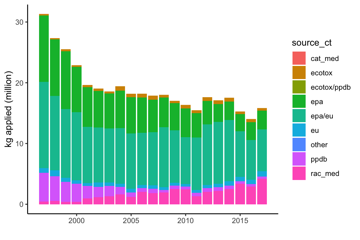
# kg applied/oral LD50 source graph
ggplot(subset(data, cat=="I" & Year<2018),
       aes(y=(kg_app/10^6), x=Year, fill=source_or)) +
  geom_col() +
  theme_classic() +
 # theme(axis.text.x=element_text(angle=90,hjust=1)) +
  ylab("kg applied (million)") +
  xlab("")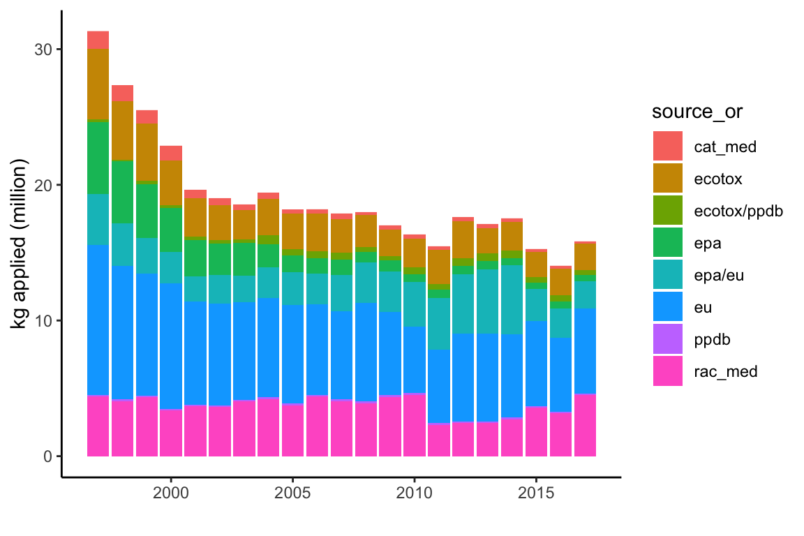
# oral source graph
ggplot(subset(data, cat=="I" & Year<2017),
       aes(y=(ld50_or_tot/10^9), x=Year, fill=source_or)) +
  geom_col() +
  theme_classic() +
  #theme(axis.text.x=element_text(angle=90,hjust=1)) +
  ylab("Oral LD50 units (billion)") +
  xlab("")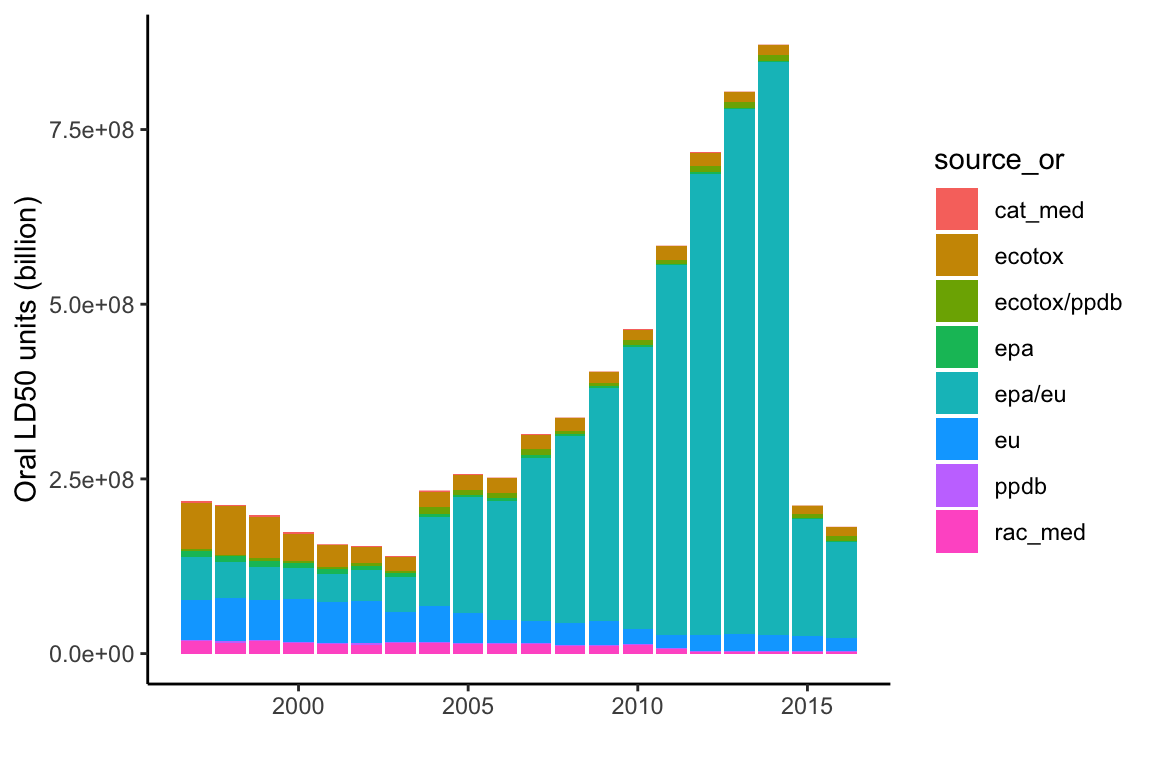
# contact source graph
ggplot(subset(data, cat=="I" & Year<2017),
       aes(y=(ld50_ct_tot/10^9), x=Year, fill=source_ct)) +
  geom_col() +
  theme_classic() +
 # theme(axis.text.x=element_text(angle=90,hjust=1)) +
  ylab("Contact LD50 units (billion)") +
  xlab("")
Examine pesticide category contributions
# kg applied graph
ggplot(subset(data, Year<2018),
       aes(y=(kg_app/10^6), x=Year, fill=cat)) +
  geom_col() +
  theme_classic() +
  theme(axis.text.x=element_text(angle=90,hjust=1)) +
  ylab("kg applied (million)")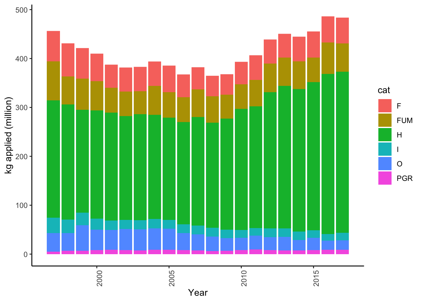
Aggregate by state-crop-year-category
data_agg_cat <- data %>%
  group_by(Year, crop, State, State_FIPS_code, STATE_ALPHA, cat) %>%
  summarise(ld50_ct_ha = sum(ld50_ct_ha, na.rm=TRUE),
            ld50_ct_tot = sum(ld50_ct_tot, na.rm=TRUE),
            ld50_or_ha = sum(ld50_or_ha, na.rm=TRUE),
            ld50_or_tot = sum(ld50_or_tot, na.rm=TRUE),
            kg_ha = sum(kg_ha, na.rm=TRUE),
            kg_app = sum(kg_app, na.rm=TRUE),
            ha = mean(ha, na.rm=TRUE))
Interpolate to fill gaps in dataset
Example
# Example interpolation

state <- "ME"
crp <- "Alfalfa"
ct <- "H"

test <- subset(data_agg_cat, crop == crp &
                   STATE_ALPHA == state &
               cat == ct) %>%
  mutate(source = "usgs")

test$pch <- NA
test$pch[test$source=="usgs"] <- 1
with(test, plot(kg_ha~Year, xlim=c(1997,2017), pch=pch))
points(approx(test$Year, test$kg_ha, method="linear", rule=2, xout=seq(1997,2017,by=1)), col=4, pch = "*")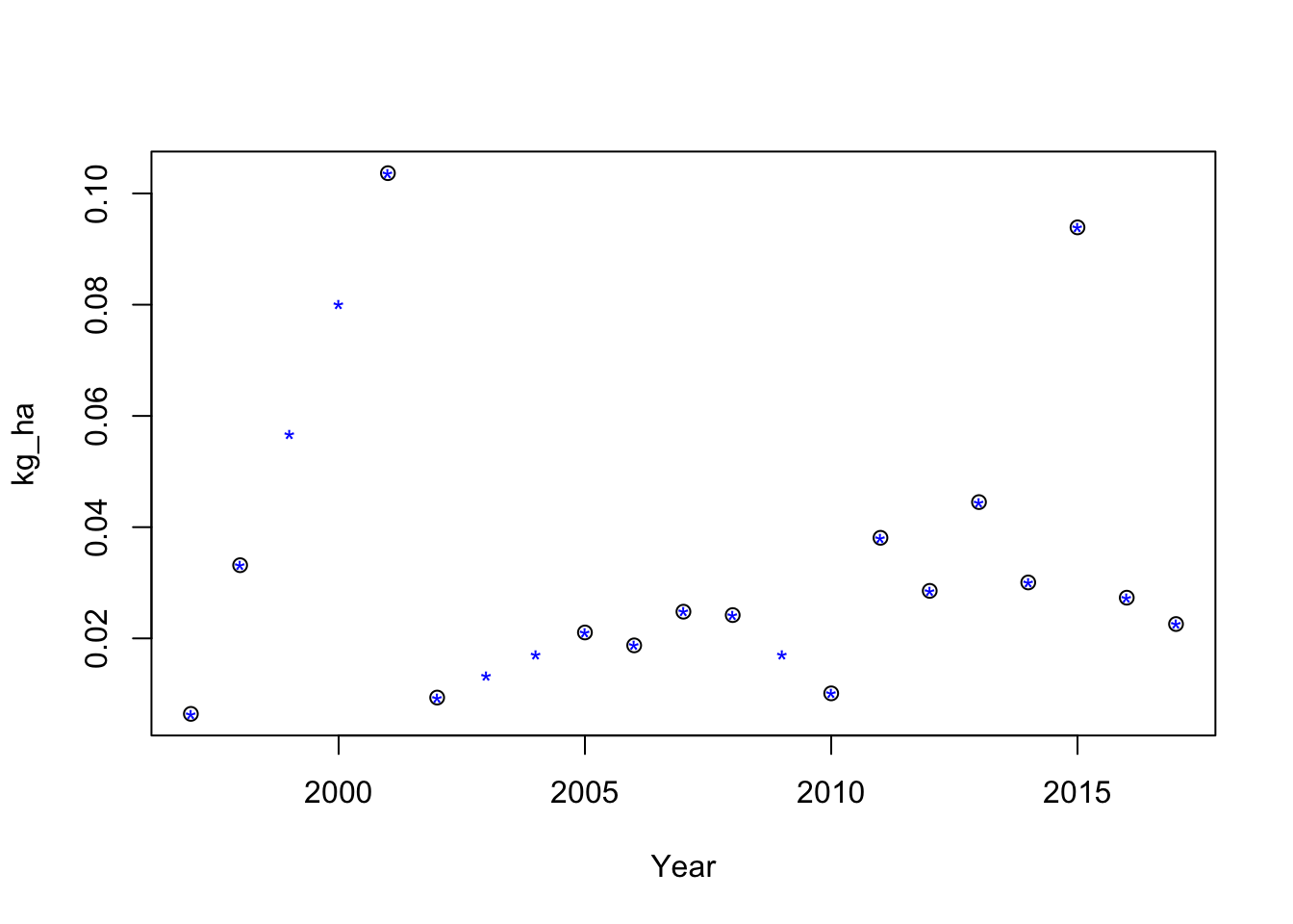
Full dataset
# Expand dataset to include all combinations of state, year, crop, category
data_agg_full <- data_agg_cat %>%
  #complete(Year, nesting(State, State_FIPS_code, STATE_ALPHA), crop, cat) %>%
  mutate(ld50_ct_ha = ifelse(cat == "I", ld50_ct_ha, NA),  # fill in NA for toxic load units for non-insecticides
         ld50_ct_tot = ifelse(cat == "I", ld50_ct_tot, NA),
         ld50_or_ha = ifelse(cat == "I", ld50_or_ha, NA),
         ld50_or_tot = ifelse(cat == "I", ld50_or_tot, NA),
         source = ifelse(!is.na(kg_app), 'usgs', NA))     # create a source column + fill in USGS if non-NA value present for kg applied

# Split data into separate dataframes by state, crop, and category
crop_state_cat <- as.factor(paste(data_agg_full$STATE_ALPHA, data_agg_full$crop, data_agg_full$cat))
crop_split_state <- split(as.data.frame(data_agg_full), f=crop_state_cat)

# Create for only insecticide data
data_agg_ins <- data_agg_cat %>%
  filter(cat == "I") %>%
  #complete(Year, nesting(State, State_FIPS_code, STATE_ALPHA), crop, cat) %>%
  mutate(source = ifelse(!is.na(kg_app), 'usgs', NA))     # create a source column + fill in USGS if non-NA value present for kg applied

# Split data into separate dataframes by state, crop, and category
crop_state_cat_ins <- as.factor(paste(data_agg_ins$STATE_ALPHA, data_agg_ins$crop, data_agg_ins$cat))
crop_split_state_ins <- split(as.data.frame(data_agg_ins), f=crop_state_cat_ins)
# This code interpolates values for missing year-state-crop combinations from 1997-2017, for those combinations that have at least two years of data, and returns a new dataframe with the original and interpolated values combined
kg_ha <- NULL
for(i in 1:length(crop_split_state))
{
if (length(crop_split_state[[i]]$kg_ha) > 1) {
df1 = crop_split_state[[i]]
temp <- as.data.frame(approx(df1$Year, df1$kg_ha, method="linear", xout=seq(1997,2017,by=1), rule=2))
temp$State <- as.character(levels(factor(df1$State)))
temp$STATE_ALPHA <- as.character(levels(factor(df1$STATE_ALPHA)))
temp$State_FIPS_code <- as.character(levels(factor(df1$State_FIPS_code)))
temp$crop <- as.character(levels(factor(df1$crop)))
temp$cat <- as.character(levels(factor(df1$cat)))
temp$interp_kg_ha <- "yes"
kg_ha <- rbind(kg_ha,temp)
}
else {
df2 = crop_split_state[[i]]
value = !is.na(crop_split_state[[i]]$kg_ha)
temp <- select(df2, Year, kg_ha, State, STATE_ALPHA, State_FIPS_code, crop, cat)
temp$interp_kg_ha <- "no"
colnames(temp)[1] <- "x"
colnames(temp)[2] <- "y"
kg_ha <- rbind(kg_ha,temp)
}
}
colnames(kg_ha)[1] <- "Year" # fix column names
colnames(kg_ha)[2] <- "kg_ha"kg_app <- NULL
for(i in 1:length(crop_split_state))
{
if (length(crop_split_state[[i]]$kg_app) > 1) {
df1 = crop_split_state[[i]]
temp <- as.data.frame(approx(df1$Year, df1$kg_app, method="linear", xout=seq(1997,2017,by=1), rule=2))
temp$State <- as.character(levels(factor(df1$State)))
temp$STATE_ALPHA <- as.character(levels(factor(df1$STATE_ALPHA)))
temp$State_FIPS_code <- as.character(levels(factor(df1$State_FIPS_code)))
temp$crop <- as.character(levels(factor(df1$crop)))
temp$cat <- as.character(levels(factor(df1$cat)))
temp$interp_kg_app <- "yes"
kg_app <- rbind(kg_app,temp)
}
else {
df2 = crop_split_state[[i]]
temp <- select(df2, Year, kg_app, State, STATE_ALPHA, State_FIPS_code, crop, cat)
colnames(temp)[1] <- "x"
colnames(temp)[2] <- "y"
temp$interp_kg_app <- "no"
kg_app <- rbind(kg_app,temp)
}
}
colnames(kg_app)[1] <- "Year" # fix column names
colnames(kg_app)[2] <- "kg_app"ld50_ct_ha <- NULL
for(i in 1:length(crop_split_state_ins))
{
if (length(crop_split_state_ins[[i]]$ld50_ct_ha) > 1) {
df1 = crop_split_state_ins[[i]]
temp <- as.data.frame(approx(df1$Year, df1$ld50_ct_ha, method="linear", xout=seq(1997,2017,by=1), rule=2))
temp$State <- as.character(levels(factor(df1$State)))
temp$STATE_ALPHA <- as.character(levels(factor(df1$STATE_ALPHA)))
temp$State_FIPS_code <- as.character(levels(factor(df1$State_FIPS_code)))
temp$crop <- as.character(levels(factor(df1$crop)))
temp$cat <- as.character(levels(factor(df1$cat)))
temp$interp_ct_ha <- "yes"
ld50_ct_ha <- rbind(ld50_ct_ha,temp)
}
else {
df2 = crop_split_state_ins[[i]]
temp <- select(df2, Year, ld50_ct_ha, State, STATE_ALPHA, State_FIPS_code, crop, cat)
colnames(temp)[1] <- "x"
colnames(temp)[2] <- "y"
temp$interp_ct_ha <- "no"
ld50_ct_ha <- rbind(ld50_ct_ha,temp)
}
}
colnames(ld50_ct_ha)[1] <- "Year" # fix column names
colnames(ld50_ct_ha)[2] <- "ld50_ct_ha"ld50_ct_tot <- NULL
for(i in 1:length(crop_split_state_ins))
{
if (length(crop_split_state_ins[[i]]$ld50_ct_tot) > 1) {
df1 = crop_split_state_ins[[i]]
temp <- as.data.frame(approx(df1$Year, df1$ld50_ct_tot, method="linear", xout=seq(1997,2017,by=1), rule=2))
temp$State <- as.character(levels(factor(df1$State)))
temp$STATE_ALPHA <- as.character(levels(factor(df1$STATE_ALPHA)))
temp$State_FIPS_code <- as.character(levels(factor(df1$State_FIPS_code)))
temp$crop <- as.character(levels(factor(df1$crop)))
temp$cat <- as.character(levels(factor(df1$cat)))
temp$interp_ct_tot <- "yes"
ld50_ct_tot <- rbind(ld50_ct_tot,temp)
}
else {
df2 = crop_split_state_ins[[i]]
temp <- select(df2, Year, ld50_ct_tot, State, STATE_ALPHA, State_FIPS_code, crop, cat)
colnames(temp)[1] <- "x"
colnames(temp)[2] <- "y"
temp$interp_ct_tot <- "no"
ld50_ct_tot <- rbind(ld50_ct_tot,temp)
}
}
colnames(ld50_ct_tot)[1] <- "Year" # fix column names
colnames(ld50_ct_tot)[2] <- "ld50_ct_tot"ld50_or_ha <- NULL
for(i in 1:length(crop_split_state_ins))
{
if (length(crop_split_state_ins[[i]]$ld50_or_ha) > 1) {
df1 = crop_split_state_ins[[i]]
temp <- as.data.frame(approx(df1$Year, df1$ld50_or_ha, method="linear", xout=seq(1997,2017,by=1), rule=2))
temp$State <- as.character(levels(factor(df1$State)))
temp$STATE_ALPHA <- as.character(levels(factor(df1$STATE_ALPHA)))
temp$State_FIPS_code <- as.character(levels(factor(df1$State_FIPS_code)))
temp$crop <- as.character(levels(factor(df1$crop)))
temp$cat <- as.character(levels(factor(df1$cat)))
temp$interp_or_ha <- "yes"
ld50_or_ha <- rbind(ld50_or_ha,temp)
}
else {
df2 = crop_split_state_ins[[i]]
temp <- select(df2, Year, ld50_or_ha, State, STATE_ALPHA, State_FIPS_code, crop, cat)
colnames(temp)[1] <- "x"
colnames(temp)[2] <- "y"
temp$interp_or_ha <- "no"
ld50_or_ha <- rbind(ld50_or_ha,temp)
}
}
colnames(ld50_or_ha)[1] <- "Year" # fix column names
colnames(ld50_or_ha)[2] <- "ld50_or_ha"ld50_or_tot <- NULL
for(i in 1:length(crop_split_state_ins))
{
if (length(crop_split_state_ins[[i]]$ld50_or_tot) > 1) {
df1 = crop_split_state_ins[[i]]
temp <- as.data.frame(approx(df1$Year, df1$ld50_or_tot, method="linear", xout=seq(1997,2017,by=1), rule=2))
temp$State <- as.character(levels(factor(df1$State)))
temp$STATE_ALPHA <- as.character(levels(factor(df1$STATE_ALPHA)))
temp$State_FIPS_code <- as.character(levels(factor(df1$State_FIPS_code)))
temp$crop <- as.character(levels(factor(df1$crop)))
temp$cat <- as.character(levels(factor(df1$cat)))
temp$interp_or_tot <- "yes"
ld50_or_tot <- rbind(ld50_or_tot,temp)
}
else {
df2 = crop_split_state_ins[[i]]
temp <- select(df2, Year, ld50_or_tot, State, STATE_ALPHA, State_FIPS_code, crop, cat)
colnames(temp)[1] <- "x"
colnames(temp)[2] <- "y"
temp$interp_or_tot <- "no"
ld50_or_tot <- rbind(ld50_or_tot,temp)
}
}
colnames(ld50_or_tot)[1] <- "Year" # fix column names
colnames(ld50_or_tot)[2] <- "ld50_or_tot"# Create a key to add sources back in
source_key <- select(as.data.frame(data_agg_full), Year, STATE_ALPHA, crop, cat, source)
# Join interpolated data with source information
data_interp <- left_join(kg_ha, source_key, by=c("STATE_ALPHA", "Year", "crop", "cat")) %>%
full_join(kg_app) %>%
full_join(ld50_ct_ha) %>%
full_join(ld50_ct_tot) %>%
full_join(ld50_or_ha) %>%
full_join(ld50_or_tot) %>%
mutate(check_kg = ifelse(interp_kg_ha == interp_kg_app, 1, 0),
check_ld50 = ifelse(interp_ct_tot == interp_or_ha, 1, 0))Joining, by = c("Year", "State", "STATE_ALPHA", "State_FIPS_code", "crop", "cat")
Joining, by = c("Year", "State", "STATE_ALPHA", "State_FIPS_code", "crop", "cat")
Joining, by = c("Year", "State", "STATE_ALPHA", "State_FIPS_code", "crop", "cat")
Joining, by = c("Year", "State", "STATE_ALPHA", "State_FIPS_code", "crop", "cat")
Joining, by = c("Year", "State", "STATE_ALPHA", "State_FIPS_code", "crop", "cat")# Replace NA source values with 'interp' to indicate interpolated
levels(data_interp$source) <- c("usgs","interp")
data_interp$source[is.na(data_interp$source)] <- "interp"
str(data_interp) # check results'data.frame': 30488 obs. of 21 variables:
$ Year : num 1997 1998 1999 2000 2001 ...
$ kg_ha : num 0.0276 0.058 0.0271 0.08 0.0369 ...
$ State : chr "Alabama" "Alabama" "Alabama" "Alabama" ...
$ STATE_ALPHA : chr "AL" "AL" "AL" "AL" ...
$ State_FIPS_code: chr "1" "1" "1" "1" ...
$ crop : chr "Alfalfa" "Alfalfa" "Alfalfa" "Alfalfa" ...
$ cat : chr "H" "H" "H" "H" ...
$ interp_kg_ha : chr "yes" "yes" "yes" "yes" ...
$ source : chr "usgs" "usgs" "usgs" "usgs" ...
..- attr(*, "levels")= chr "usgs" "interp"
$ kg_app : num 146 297 134 381 169 ...
$ interp_kg_app : chr "yes" "yes" "yes" "yes" ...
$ ld50_ct_ha : num NA NA NA NA NA NA NA NA NA NA ...
$ interp_ct_ha : chr NA NA NA NA ...
$ ld50_ct_tot : num NA NA NA NA NA NA NA NA NA NA ...
$ interp_ct_tot : chr NA NA NA NA ...
$ ld50_or_ha : num NA NA NA NA NA NA NA NA NA NA ...
$ interp_or_ha : chr NA NA NA NA ...
$ ld50_or_tot : num NA NA NA NA NA NA NA NA NA NA ...
$ interp_or_tot : chr NA NA NA NA ...
$ check_kg : num 1 1 1 1 1 1 1 1 1 1 ...
$ check_ld50 : num NA NA NA NA NA NA NA NA NA NA ...# Fill in values for singletons
data_singles <- filter(data_interp, interp_kg_app == "no") %>%
select(STATE_ALPHA, crop, cat,
kg_app_s = kg_app,
kg_ha_s = kg_ha,
ld50_ct_ha_s = ld50_ct_ha,
ld50_ct_tot_s = ld50_ct_tot,
ld50_or_ha_s = ld50_or_ha,
ld50_or_tot_s = ld50_or_tot)
data_interp_full <- data_interp %>%
complete(Year, nesting(State, State_FIPS_code, STATE_ALPHA), nesting(crop, cat)) %>%
left_join(data_singles, by = c('STATE_ALPHA', 'crop', 'cat')) %>%
mutate(source = ifelse(!is.na(kg_app), source,
ifelse(!is.na(kg_app_s), "interp_s", NA)),
kg_app = ifelse(!is.na(kg_app), kg_app,
ifelse(!is.na(kg_app_s), kg_app_s, NA)),
kg_ha = ifelse(!is.na(kg_ha), kg_ha,
ifelse(!is.na(kg_ha_s), kg_ha_s, NA)),
ld50_ct_ha = ifelse(!is.na(ld50_ct_ha), ld50_ct_ha,
ifelse(!is.na(ld50_ct_ha_s), ld50_ct_ha_s, NA)),
ld50_ct_tot = ifelse(!is.na(ld50_ct_tot), ld50_ct_tot,
ifelse(!is.na(ld50_ct_tot_s), ld50_ct_tot_s, NA)),
ld50_or_ha = ifelse(!is.na(ld50_or_ha), ld50_or_ha,
ifelse(!is.na(ld50_or_ha_s), ld50_or_ha_s, NA)),
ld50_or_tot = ifelse(!is.na(ld50_or_tot), ld50_or_tot,
ifelse(!is.na(ld50_or_tot_s), ld50_or_tot_s, NA))
) %>%
filter(!is.na(kg_ha))
# Create a key to add ha back in
ha_key <- select(as.data.frame(data_agg_full), Year, STATE_ALPHA, crop, cat, ha)
# Generate clean dataset
data_clean <- data_interp_full %>%
select(Year, State, STATE_ALPHA, State_FIPS_code, crop, cat, kg_app, kg_ha, ld50_ct_ha, ld50_ct_tot, ld50_or_ha, ld50_or_tot, source) %>%
left_join(ha_key, by = c("STATE_ALPHA", "Year", "crop", "cat")) %>%
filter(cat != "I" | Year < 2015) # remove insecticide data post-2014
str(data_clean)Classes 'tbl_df', 'tbl' and 'data.frame': 33468 obs. of 14 variables:
$ Year : num 1997 1997 1997 1997 1997 ...
$ State : chr "Alabama" "Alabama" "Alabama" "Alabama" ...
$ STATE_ALPHA : chr "AL" "AL" "AL" "AL" ...
$ State_FIPS_code: chr "1" "1" "1" "1" ...
$ crop : chr "Alfalfa" "Alfalfa" "Corn" "Corn" ...
$ cat : chr "H" "I" "F" "H" ...
$ kg_app : num 146 304 325 389024 6394 ...
$ kg_ha : num 0.0276 0.0574 0.0031 3.6956 0.0607 ...
$ ld50_ct_ha : num NA 1.05e+09 NA NA 3.80e+08 ...
$ ld50_ct_tot : num NA 5.57e+12 NA NA 4.00e+13 ...
$ ld50_or_ha : num NA 6.78e+08 NA NA 1.48e+08 ...
$ ld50_or_tot : num NA 3.59e+12 NA NA 1.56e+13 ...
$ source : chr "usgs" "usgs" "interp" "usgs" ...
$ ha : num 5297 5297 NA 105266 105266 ...summary(data_clean) Year State STATE_ALPHA State_FIPS_code
Min. :1997 Length:33468 Length:33468 Length:33468
1st Qu.:2002 Class :character Class :character Class :character
Median :2007 Mode :character Mode :character Mode :character
Mean :2007
3rd Qu.:2012
Max. :2017
crop cat kg_app
Length:33468 Length:33468 Min. : 0
Class :character Class :character 1st Qu.: 409
Mode :character Mode :character Median : 5861
Mean : 260983
3rd Qu.: 52999
Max. :34908487
kg_ha ld50_ct_ha ld50_ct_tot
Min. : 0.0000 Min. :0.000e+00 Min. :0.000e+00
1st Qu.: 0.0057 1st Qu.:1.423e+08 1st Qu.:8.302e+12
Median : 0.0938 Median :9.201e+08 Median :4.913e+13
Mean : 2.2020 Mean :5.054e+09 Mean :5.016e+14
3rd Qu.: 1.5718 3rd Qu.:4.973e+09 3rd Qu.:2.715e+14
Max. :365.3683 Max. :1.770e+11 Max. :2.145e+16
NA's :26628 NA's :26628
ld50_or_ha ld50_or_tot source
Min. :0.000e+00 Min. :0.000e+00 Length:33468
1st Qu.:8.730e+07 1st Qu.:6.828e+12 Class :character
Median :1.468e+09 Median :5.291e+13 Mode :character
Mean :6.730e+09 Mean :9.551e+14
3rd Qu.:8.062e+09 3rd Qu.:3.858e+14
Max. :1.439e+11 Max. :7.374e+16
NA's :26628 NA's :26628
ha
Min. : 51
1st Qu.: 7898
Median : 59894
Mean : 525116
3rd Qu.: 265348
Max. :43921050
NA's :9525 table(data_clean$source)
  interp interp_s     usgs
    5549     3976    23943
Examine patterns in data
Graph by USGS group to check interpolation
# Split dataset by crop
data_graph <- data_clean %>%
  mutate(cat_crop = paste(cat, crop)) %>%
  filter(cat %in% c("I","H","F"))

data_graph2 <- data_clean %>%
  mutate(cat_crop = paste(cat, crop)) %>%
  filter(cat == "I")

group_state_split <- split(as.data.frame(data_graph), f = data_graph$cat_crop)

group_state_split2 <- split(as.data.frame(data_graph2), f = data_graph2$cat_crop)

colors <- c(usgs = "black", interp = "dodgerblue", interp_s = "darkorchid1")

pdf("../output/kg_ha-by-state-yr.pdf",
    width=12, height=8)
for(i in 1:length(group_state_split))
{
  df1 = as.data.frame(group_state_split[[i]])
  plot <- ggplot(df1, aes(x=Year, y = kg_ha, colour = source)) +
            geom_point() +
            ylab("kg/ha") + xlab("") +
            facet_wrap(~STATE_ALPHA) +
            scale_colour_manual(values = colors) +
            ggtitle(levels(factor(df1$cat_crop))) +
            theme_classic()
  print(plot)
}
dev.off()

pdf("../output/ld50_or-by-state-yr.pdf",
    width=12, height=8)
for(i in 1:length(group_state_split2))
{
  df1 = as.data.frame(group_state_split2[[i]])
  plot <- ggplot(df1, aes(x=Year, y = ld50_or_ha/10^9, colour = source)) +
            geom_point() +
            ylab("bil oral LD50/ha") + xlab("") +
            facet_wrap(~STATE_ALPHA) +
            scale_colour_manual(values = colors) +
            ggtitle(levels(factor(df1$cat_crop))) +
            theme_classic()
  print(plot)
}
dev.off()

pdf("../output/ld50_ct-by-state-yr.pdf",
    width=12, height=8)
for(i in 1:length(group_state_split2))
{
  df1 = as.data.frame(group_state_split2[[i]])
  plot <- ggplot(df1, aes(x=Year, y = ld50_ct_ha/10^9, colour = source)) +
            geom_point() +
            ylab("bil contact LD50/ha") + xlab("") +
            facet_wrap(~STATE_ALPHA) +
            scale_colour_manual(values = colors) +
            ggtitle(levels(factor(df1$cat_crop))) +
            theme_classic()
  print(plot)
}
dev.off()
Patterns by state
# kg applied by crop
ggplot(subset(data_clean, cat=="I" & Year<2018 & !is.na(STATE_ALPHA)),
       aes(y=(kg_app/10^6), x=Year, fill=crop)) +
  geom_col() +
  theme_classic() +
  theme(axis.text.x=element_text(angle=90,hjust=1)) +
  ylab("kg applied (mil)") +
  facet_wrap(~STATE_ALPHA, scales="free_y")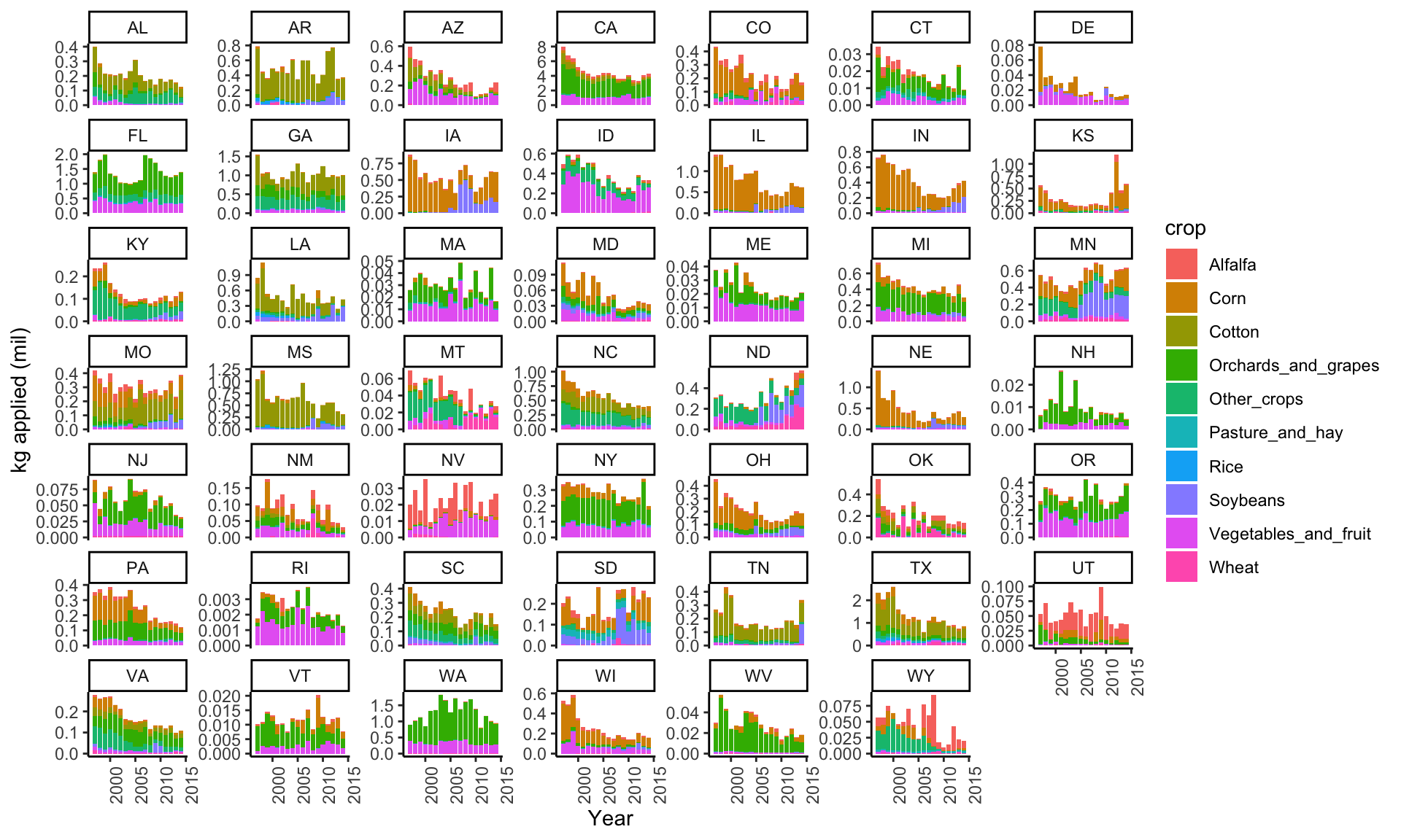
# contact LD50 by crop
ggplot(subset(data_clean, cat=="I" & Year<2018 & !is.na(STATE_ALPHA)),
       aes(y=(ld50_ct_tot/10^12), x=Year, fill=crop)) +
  geom_col() +
  theme_classic() +
  theme(axis.text.x=element_text(angle=90,hjust=1)) +
  ylab("Contact LD50 units (tril)") +
  facet_wrap(~STATE_ALPHA, scales="free_y")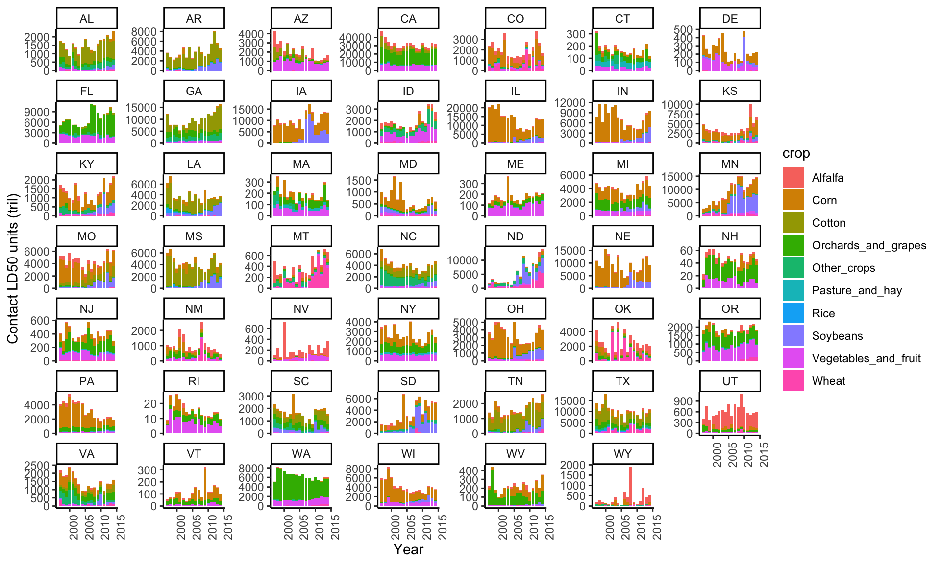
# oral LD50 by crop
ggplot(subset(data_clean, cat=="I" & Year<2018 & !is.na(STATE_ALPHA)),
       aes(y=(ld50_or_tot/10^12), x=Year, fill=crop)) +
  geom_col() +
  theme_classic() +
  theme(axis.text.x=element_text(angle=90,hjust=1)) +
  ylab("Oral LD50 units (tril)") +
  facet_wrap(~STATE_ALPHA, scales="free_y")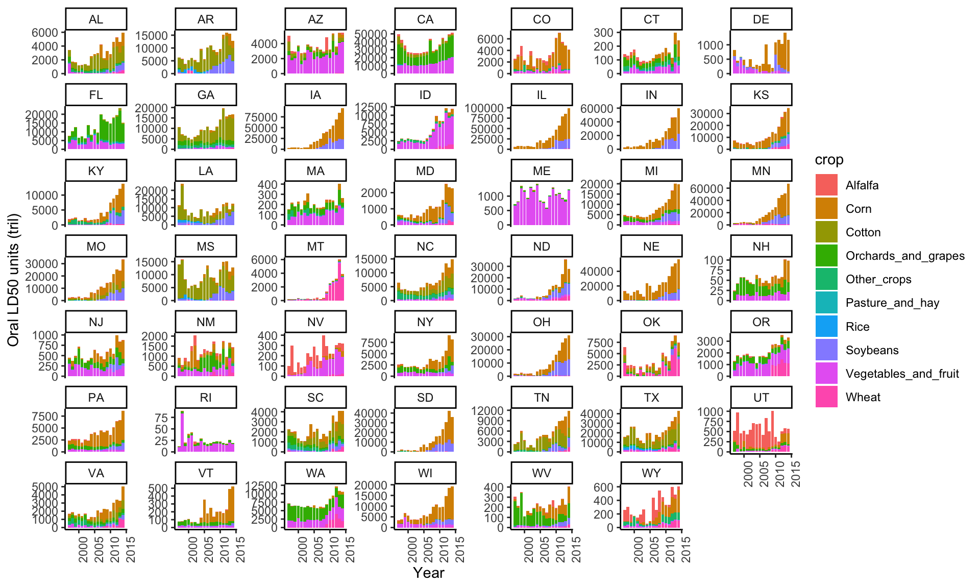
Export data
write.csv(data_clean,"../output_big/bee_tox_index_state_yr_cat_20210625.csv", row.names=FALSE)
write.csv(data,"../output_big/bee_tox_index_state_yr_cmpd_20200609.csv", row.names=FALSE)
Session information
sessionInfo()R version 3.6.1 (2019-07-05)
Platform: x86_64-apple-darwin15.6.0 (64-bit)
Running under: macOS Catalina 10.15.7
Matrix products: default
BLAS: /Library/Frameworks/R.framework/Versions/3.6/Resources/lib/libRblas.0.dylib
LAPACK: /Library/Frameworks/R.framework/Versions/3.6/Resources/lib/libRlapack.dylib
locale:
[1] en_US.UTF-8/en_US.UTF-8/en_US.UTF-8/C/en_US.UTF-8/en_US.UTF-8
attached base packages:
[1] stats graphics grDevices utils datasets methods base
other attached packages:
[1] forcats_0.4.0 stringr_1.4.0 dplyr_0.8.3 purrr_0.3.2
[5] readr_1.3.1 tidyr_1.1.0 tibble_2.1.3 ggplot2_3.2.0
[9] tidyverse_1.2.1
loaded via a namespace (and not attached):
[1] Rcpp_1.0.6 cellranger_1.1.0 pillar_1.4.2 compiler_3.6.1
[5] tools_3.6.1 digest_0.6.20 lubridate_1.7.4 jsonlite_1.6
[9] evaluate_0.14 lifecycle_0.2.0 nlme_3.1-140 gtable_0.3.0
[13] lattice_0.20-38 pkgconfig_2.0.2 rlang_0.4.7 cli_1.1.0
[17] rstudioapi_0.10 yaml_2.2.0 haven_2.1.1 xfun_0.8
[21] withr_2.1.2 xml2_1.2.0 httr_1.4.2 knitr_1.23
[25] hms_0.5.0 generics_0.0.2 vctrs_0.3.2 grid_3.6.1
[29] tidyselect_1.1.0 glue_1.3.1 R6_2.4.0 readxl_1.3.1
[33] rmarkdown_1.14 modelr_0.1.4 magrittr_1.5 ellipsis_0.2.0.1
[37] backports_1.1.4 scales_1.0.0 htmltools_0.3.6 rvest_0.3.4
[41] assertthat_0.2.1 colorspace_1.4-1 labeling_0.3 stringi_1.4.3
[45] lazyeval_0.2.2 munsell_0.5.0 broom_0.5.2 crayon_1.3.4 This R Markdown site was created with workflowr